Ex 6: Numbers-at-age / survival deviations as random effects
Source:vignettes/ex06_NAA.Rmd
ex06_NAA.RmdIn this vignette we walk through an example using the
wham (WHAM = Woods Hole Assessment Model) package to run a
state-space age-structured stock assessment model. WHAM is a
generalization of code written for Miller et al. (2016)
and Xu et
al. (2018), and in this example we apply WHAM to the same stock,
Southern New England / Mid-Atlantic Yellowtail Flounder.
This is the 6th WHAM example, which blends aspects from Ex
1, Ex
2, and Ex
5. We assume you already have wham installed. If not,
see the Introduction.
The simpler 1st example is available as a R
script and vignette.
As in example 1:
- Stock: Southern New England-Mid Atlantic (SNEMA) yellowtail flounder
- Data: 1973-2011, 1 fishery and 2 indices
- Age compositions: logistic normal, treating observations of zero as
missing (
age_comp = "logistic-normal-miss0") - Selectivity: age-specific
As in example 2:
- Beverton-Holt recruitment (
recruit_model = 3) - Environmental covariate (ecov) modeled as an AR1 process
(
ecov$process_model = 'ar1') - Compare with and w/o ecov having a “limiting” (carrying capacity)
effect on recruitment (
ecov$how = 2)
As in example 4:
- Age-specific selectivity with some ages fixed at 1 (fishery: 4-5, index1: 4, index2: 2-4)
As in example 5:
- Environmental covariate: Gulf Stream Index (GSI)
- 2D AR1 deviations by age and year (random effects)
Example 6 highlights WHAM’s options for treating the yearly transitions in numbers-at-age (i.e. survival):
- Deterministic (as in statistical catch-at-age models, recruitment in each year estimated as independent fixed effect parameters)
- Recruitment deviations (from Bev-Holt expectation) are random
effects
- independent
- AR1 deviations by year (autocorrelated)
- “Full state-space model” (survival of all ages are random effects)
- independent
- AR1 deviations by age
- AR1 deviations by year
- 2D AR1 deviations by age and year
1. Load data
Open R and load wham and other useful packages:
For a clean, runnable .R script, look at
ex6_NAA.R in the example_scripts folder of the
wham package. You can run this entire example script
with:
wham.dir <- find.package("wham")
source(file.path(wham.dir, "example_scripts", "ex6_NAA.R"))
Let’s create a directory for this analysis:
# choose a location to save output, otherwise will be saved in working directory
write.dir <- "choose/where/to/save/output" # need to change e.g., tempdir(check=TRUE)
dir.create(write.dir)
setwd(write.dir)
We need the same ASAP data file as in example
1, and the environmental covariate (Gulf Stream Index, GSI). Read in
ex1_SNEMAYT.dat and GSI.csv:
asap3 <- read_asap3_dat(file.path(wham.dir,"extdata","ex2_SNEMAYT.dat"))
env.dat <- read.csv(file.path(wham.dir,"extdata","GSI.csv"), header=T)
head(env.dat)
As in example 5, the GSI data file does not have a standard error estimate, either for each yearly observation or one overall value. In such a case, WHAM can estimate the observation error for the environmental covariate, either as one overall value, , or yearly values as random effects, . In this example we choose the simpler option and estimate one observation error parameter, shared across years.
2. Specify models
Now we specify several models with different options for the numbers-at-age (NAA) transitions, i.e. survival:
df.mods <- data.frame(NAA_cor = c('---','iid','ar1_y','iid','ar1_a','ar1_y','2dar1','iid','ar1_y','iid','ar1_a','ar1_y','2dar1'),
                      NAA_sigma = c('---',rep("rec",2),rep("rec+1",4),rep("rec",2),rep("rec+1",4)),
                      R_how = paste0(c(rep("none",7),rep("limiting-lag-1-linear",6))), stringsAsFactors=FALSE)
n.mods <- dim(df.mods)[1]
df.mods$Model <- paste0("m",1:n.mods)
df.mods <- df.mods |> select(Model, everything()) # moves Model to first col
Look at the model table:
df.mods
#>    Model NAA_cor NAA_sigma                 R_how
#> 1     m1     ---       ---                  none
#> 2     m2     iid       rec                  none
#> 3     m3   ar1_y       rec                  none
#> 4     m4     iid     rec+1                  none
#> 5     m5   ar1_a     rec+1                  none
#> 6     m6   ar1_y     rec+1                  none
#> 7     m7   2dar1     rec+1                  none
#> 8     m8     iid       rec limiting-lag-1-linear
#> 9     m9   ar1_y       rec limiting-lag-1-linear
#> 10   m10     iid     rec+1 limiting-lag-1-linear
#> 11   m11   ar1_a     rec+1 limiting-lag-1-linear
#> 12   m12   ar1_y     rec+1 limiting-lag-1-linear
#> 13   m13   2dar1     rec+1 limiting-lag-1-linear
3. Numbers-at-age options
To specify the options for modeling NAA transitions, include an
optional list argument, NAA_re, to the
prepare_wham_input function (see the
prepare_wham_input help page). ASAP3 does not estimate
random effects, and therefore these options are not specified in the
ASAP data file. By default (NAA_re is NULL or
not included), WHAM fits a traditional statistical catch-at-age model
(NAA = predicted NAA for all ages, i.e. survival is deterministic). To
fit a state-space model, we must specify NAA_re.
NAA_re is a list with the following entries:
-
$sigma: Which ages allow deviations from pred_NAA? Common options are specified with strings.-
"rec": Recruitment deviations are random effects, survival of all other ages is deterministic -
"rec+1": Survival of all ages is stochastic (“full state space model”), with 2 estimated , one for recruitment and one shared among other ages
-
-
$cor: Correlation structure for the NAA deviations. Options are:-
"iid": NAA deviations vary by year and age, but uncorrelated. -
"ar1_a": NAA deviations correlated by age (AR1). -
"ar1_y": NAA deviations correlated by year (AR1). -
"2dar1": NAA deviations correlated by year and age (2D AR1, as for in example 5).
-
Alternatively, you can specify a more complex configuration of sigma
parameter estimation via NAA_re$sigma_map as an array
(n_stocks x n_regions x n_ages) of integers (and NAs to fix parameters).
For example (with 1 stock and 1 region here),
NAA_re$sigma = array(c(1,2,2,3,3,3), dim = c(1,1,6)) will
estimate three
parameters, with recruitment (age-1) deviations having their own
,
ages 2-3 sharing
,
and ages 4-6 sharing
.
To fit model m1 (SCAA) we do not have to supply
anything:
NAA_re <- NULL # or simply leave out of call to prepare_wham_inputTo fit model m3, recruitment deviations are correlated
random effects:
NAA_re <- list(sigma="rec", cor="ar1_y")And to fit model m7, numbers at all ages are random
effects correlated by year AND age:
NAA_re <- list(sigma="rec+1", cor="2dar1")4. Linking recruitment to an environmental covariate (GSI)
As described in example
2, the environmental covariate options are fed to
prepare_wham_input as a list, ecov. This
example differs from example 2 in that:
-
ecov$logsigma = "est_1"estimates the GSI observation error (, one overall value for all years like in example 5). The other option is"est_re"to allow the GSI observation error to have yearly fluctuations (random effects). The Cold Pool Index in example 2 had yearly observation errors given, so this was not necessary. -
ecov$R_how = matrix("none",1,1)orecov$R_how = NULLestimates the GSI time-series model (AR1) for models without a GSI-Recruitment effect, in order to compare AIC with models that do include the effect. Settingecov$R_how = matrix("limiting-lag-1-linear,1,1)specifies that the GSI in year affects the Beverton-Holt parameter (“limiting” / carrying capacity effect) in year linearly (on log scale).
For example, the ecov list for models
m8-m13 with the linear
GSI-
effect:
  ecov <- list(
    label = "GSI",
    mean = as.matrix(env.dat$GSI),
    logsigma = 'est_1', # estimate obs sigma, 1 value shared across years
    year = env.dat$year,
    use_obs = matrix(1, ncol=1, nrow=dim(env.dat)[1]), # use all obs (=1)
    process_model = 'ar1', # "rw" or "ar1"
    R_how = matrix("limiting-lag-1-linear",1,1)) # n_Ecov x n_stocks x n_ages x n_regions
Note that you can set ecov = NULL to fit the model
without environmental covariate data, but here we fit the
ecov data even for models without the GSI effect on
recruitment (m1-m7) so that we can compare
them via AIC (need to have the same data in the likelihood). We
accomplish this by setting ecov$R_how = matrix("none",1,1)
and ecov$process_model = "ar1".
5. Run all models
All models use the same options for expected recruitment (Beverton-Holt stock-recruit function) and selectivity (age-specific, with one or two ages fixed at 1). We specify recruitment decoupling only for consistency with the original implicit assumption in WHAM.
mods <- vector("list",n.mods)
for(m in 1:n.mods){
  NAA_list <- list(cor=df.mods[m,"NAA_cor"], sigma=df.mods[m,"NAA_sigma"], decouple_recruitment = FALSE)
  if(NAA_list$sigma == '---') NAA_list = NULL

  ecov <- list(
    label = "GSI",
    mean = as.matrix(env.dat$GSI),
    logsigma = 'est_1', # estimate obs sigma, 1 value shared across years
    year = env.dat$year,
    use_obs = matrix(1, ncol=1, nrow=dim(env.dat)[1]), # use all obs (=1)
    process_model = 'ar1', # "rw" or "ar1"
    recruitment_how = matrix(df.mods$R_how[m])) # n_Ecov x n_stocks

  input <- suppressWarnings(prepare_wham_input(asap3, recruit_model = 3, # Bev Holt recruitment
                              model_name = "Ex 6: Numbers-at-age",
                              selectivity=list(model=rep("age-specific",3), re=c("none","none","none"),
                                initial_pars=list(c(0.1,0.5,0.5,1,1,1),c(0.5,0.5,0.5,1,0.5,0.5),c(0.5,0.5,1,1,1,1)),
                                fix_pars=list(4:6,4,3:6)),
                              NAA_re = NAA_list,
                              ecov=ecov,
                              age_comp = "logistic-normal-miss0")) # logistic normal, treat 0 obs as missing

  # Fit model
  mods[[m]] <- fit_wham(input, do.retro=T, do.osa=F)

  # Save model
  saveRDS(mods[[m]], file=paste0(df.mods$Model[m],".rds"))

  # If desired, do projections
  # mod_proj <- project_wham(mod)
  # saveRDS(mod_proj, file=paste0(df.mods$Model[m],"_proj.rds"))
}
6. Compare models
Get model convergence and stats.
opt_conv = 1-sapply(mods, function(x) x$opt$convergence)
ok_sdrep = sapply(mods, function(x) if(x$na_sdrep==FALSE & !is.na(x$na_sdrep)) 1 else 0)
df.mods$conv <- as.logical(opt_conv)
df.mods$pdHess <- as.logical(ok_sdrep)
Only calculate AIC and Mohn’s rho for converged models.
df.mods$runtime <- sapply(mods, function(x) x$runtime)
df.mods$NLL <- sapply(mods, function(x) round(x$opt$objective,3))
not_conv <- !df.mods$conv | !df.mods$pdHess
mods2 <- mods
mods2[not_conv] <- NULL
df.aic.tmp <- as.data.frame(compare_wham_models(mods2, table.opts=list(sort=FALSE, calc.rho=TRUE))$tab)
df.aic <- df.aic.tmp[FALSE,]
ct = 1
for(i in 1:n.mods){
  if(not_conv[i]){
    df.aic[i,] <- rep(NA,5)
  } else {
    df.aic[i,] <- df.aic.tmp[ct,]
    ct <- ct + 1
  }
}
df.aic[,1:2] <- format(round(df.aic[,1:2], 1), nsmall=1)
df.aic[,3:5] <- format(round(df.aic[,3:5], 3), nsmall=3)
df.aic[grep("NA",df.aic$dAIC),] <- "---"
df.mods <- cbind(df.mods, df.aic)
rownames(df.mods) <- NULL
Look at results table.
df.modsSave results table.
write.csv(df.mods, file="ex6_table.csv",quote=F, row.names=F)Plot output for models that converged.
mods[[1]]$env$data$recruit_model = 2 # m1 (SCAA) didn't actually fit a Bev-Holt
for(m in which(!not_conv)){
  plot_wham_output(mod=mods[[m]], dir.main=file.path(getwd(),paste0("m",m))) #html by default
}
7. Results
Two models had very similar AIC and were overwhelmingly supported
relative to the other models (bold in table below):
m11 (all NAA are random effects with correlation by age,
GSI-Recruitment effect) and m13 (all NAA are random effects
with correlation by age and year, GSI-Recruitment effect).
The SCAA and state-space models with independent NAA deviations had
the lowest runtime. Estimating NAA deviations only for age-1,
i.e. recruitment as random effects, broke the Hessian sparseness, making
models m2, m3, m8, and
m9 the slowest. Adding correlation structure to the NAA
deviations increased runtime roughly 50% (comparing models
m4 with m5-m7 and
m10 with m11-m13).
All models except for m3 converged and successfully
inverted the Hessian to produce SE estimates for (fixed effect)
parameters. Inspection of the fixed effects parameter estimates shows
that 2 of the logit transformed selectivity parameters are large
implying selectivity of 1 for those ages. Fixing those parameters at 1
probably would correct this issue. WHAM stores information about hessian
invertibility in mod$na_sdrep (should be
FALSE), mod$sdrep$pdHess (should be
TRUE). Also, mod$opt$convergence should
generally be 0. See stats::nlminb() and
TMB::sdreport() for details.
AIC for model m1 is not comparable with other models
because comparing models in which parameters (here, recruitment
deviations) are estimated as fixed effects versus random effects is
messy and marginal AIC is not appropriate. Still, we include
m1 to show 1) that WHAM can fit this NAA option, and 2) the
poor retrospective pattern in the status quo assessment. Note that
m2 is identical to m1 except that recruitment
deviations are random effects instead of fixed effects. The
retrospective patterns are very similar, but m2 takes about
3x longer to run.
| Model | NAA_cor | NAA_sigma | R_how | Converged | PD Hessian | Runtime (min) | NLL | AIC | ||||
|---|---|---|---|---|---|---|---|---|---|---|---|---|
| m1 | — | — | none | TRUE | TRUE | 0.32 | -623.530 | — | — | 8.818 | 0.951 | -0.433 |
| m2 | iid | rec | none | TRUE | TRUE | 0.92 | -509.511 | 512.2 | -875.0 | 5.054 | 1.023 | -0.437 |
| m3 | ar1_y | rec | none | TRUE | FALSE | 0.96 | -527.116 | — | — | — | — | — |
| m4 | iid | rec+1 | none | TRUE | TRUE | 0.59 | -745.447 | 42.3 | -1344.9 | 0.423 | 0.068 | -0.058 |
| m5 | ar1_a | rec+1 | none | TRUE | TRUE | 0.61 | -759.028 | 17.1 | -1370.1 | 0.240 | 0.030 | -0.039 |
| m6 | ar1_y | rec+1 | none | TRUE | TRUE | 0.73 | -753.699 | 27.8 | -1359.4 | 0.437 | 0.036 | -0.017 |
| m7 | 2dar1 | rec+1 | none | TRUE | TRUE | 0.73 | -763.264 | 10.7 | -1376.5 | 0.249 | 0.015 | -0.020 |
| m8 | iid | rec | limiting-lag-1-linear | TRUE | TRUE | 1.02 | -520.571 | 492.1 | -895.1 | 1.867 | 1.026 | -0.426 |
| m9 | ar1_y | rec | limiting-lag-1-linear | TRUE | TRUE | 1.01 | -531.190 | 472.8 | -914.4 | 2.293 | 1.008 | -0.439 |
| m10 | iid | rec+1 | limiting-lag-1-linear | TRUE | TRUE | 0.59 | -754.897 | 25.4 | -1361.8 | 0.299 | 0.052 | -0.042 |
| m11 | ar1_a | rec+1 | limiting-lag-1-linear | TRUE | TRUE | 0.80 | -767.876 | 1.4 | -1385.8 | 0.166 | 0.021 | -0.027 |
| m12 | ar1_y | rec+1 | limiting-lag-1-linear | TRUE | TRUE | 0.67 | -759.243 | 18.7 | -1368.5 | 0.277 | 0.031 | -0.014 |
| m13 | 2dar1 | rec+1 | limiting-lag-1-linear | TRUE | TRUE | 0.86 | -769.605 | 0.0 | -1387.2 | 0.142 | 0.011 | -0.016 |
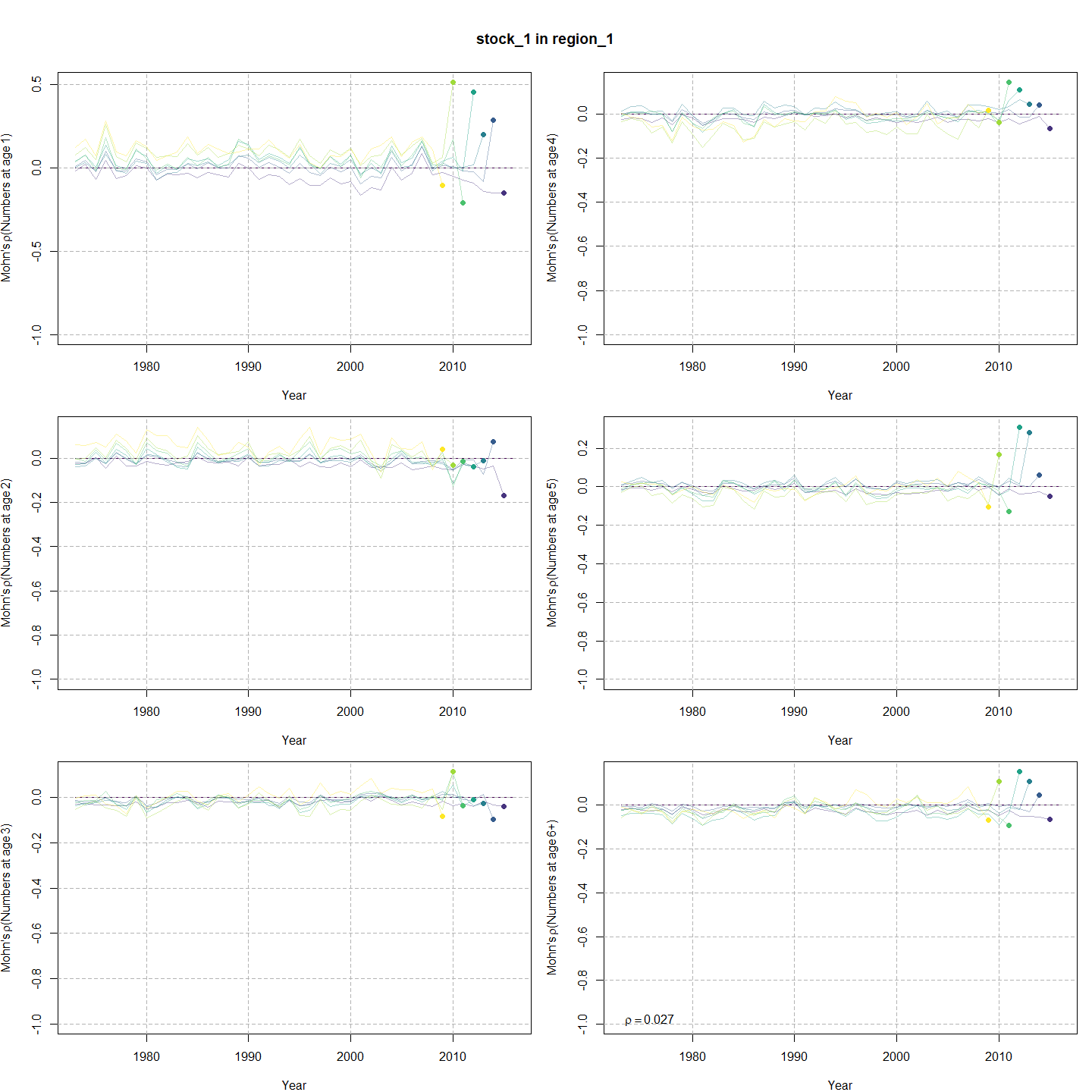
Estimated NAA deviations
- All models estimated positive recruitment (age-1) deviations in the 1970s and 80s (red), and more negative deviations since 1990 (blue).
- Models with all numbers-at-age as random effects estimated less extreme recruitment deviations (lighter red and blue for age 1).
- Models with a GSI-Recruitment link also had less extreme recruitment deviations, because the GSI effect on expected recruitment accounted for some of this variability.
Estimated survival deviations by age (y-axis) and year (x-axis) for
all converged models: 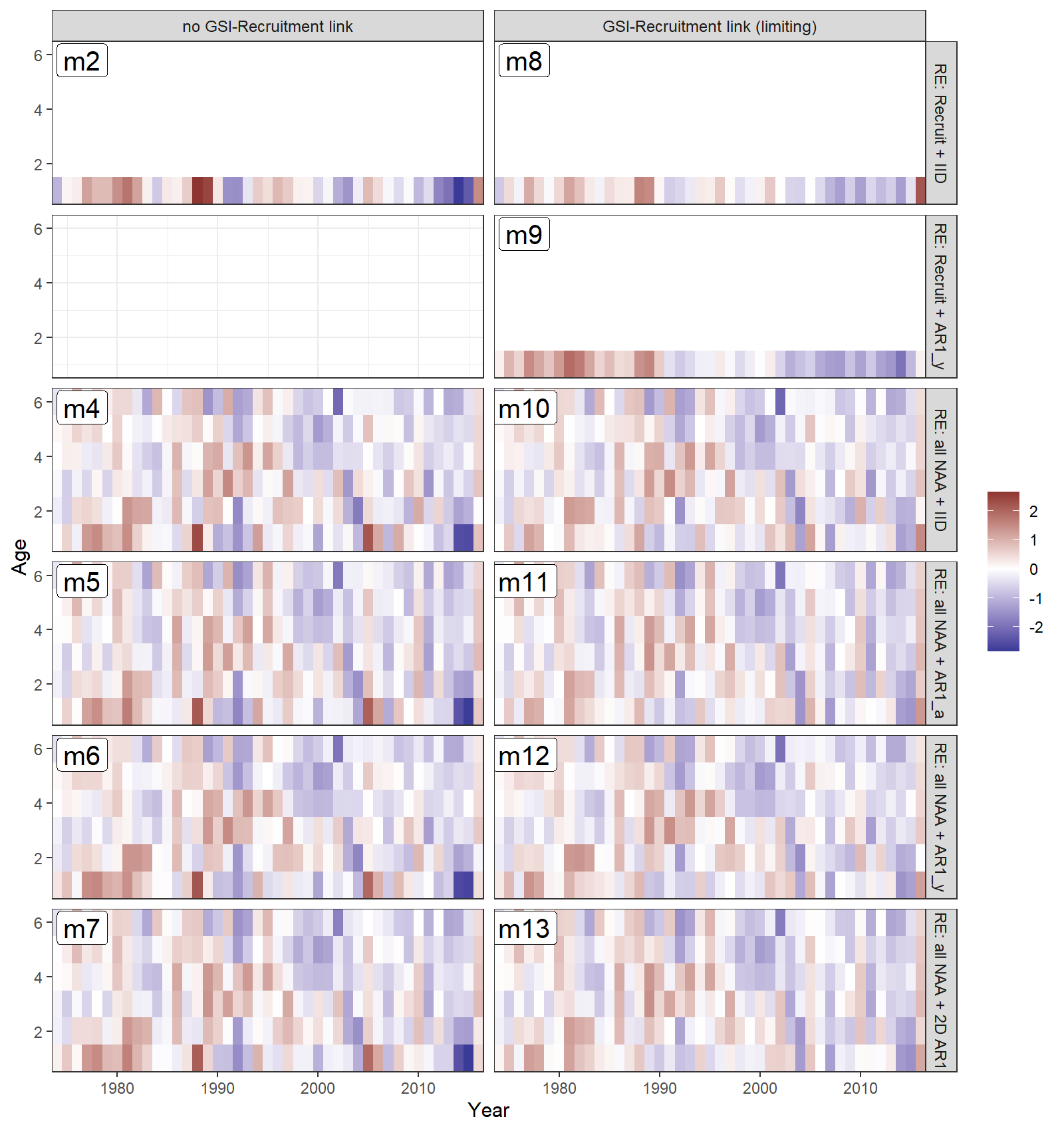
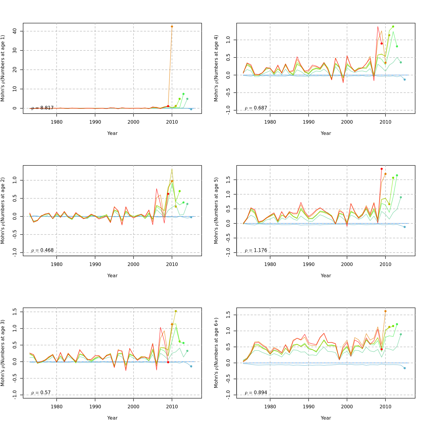
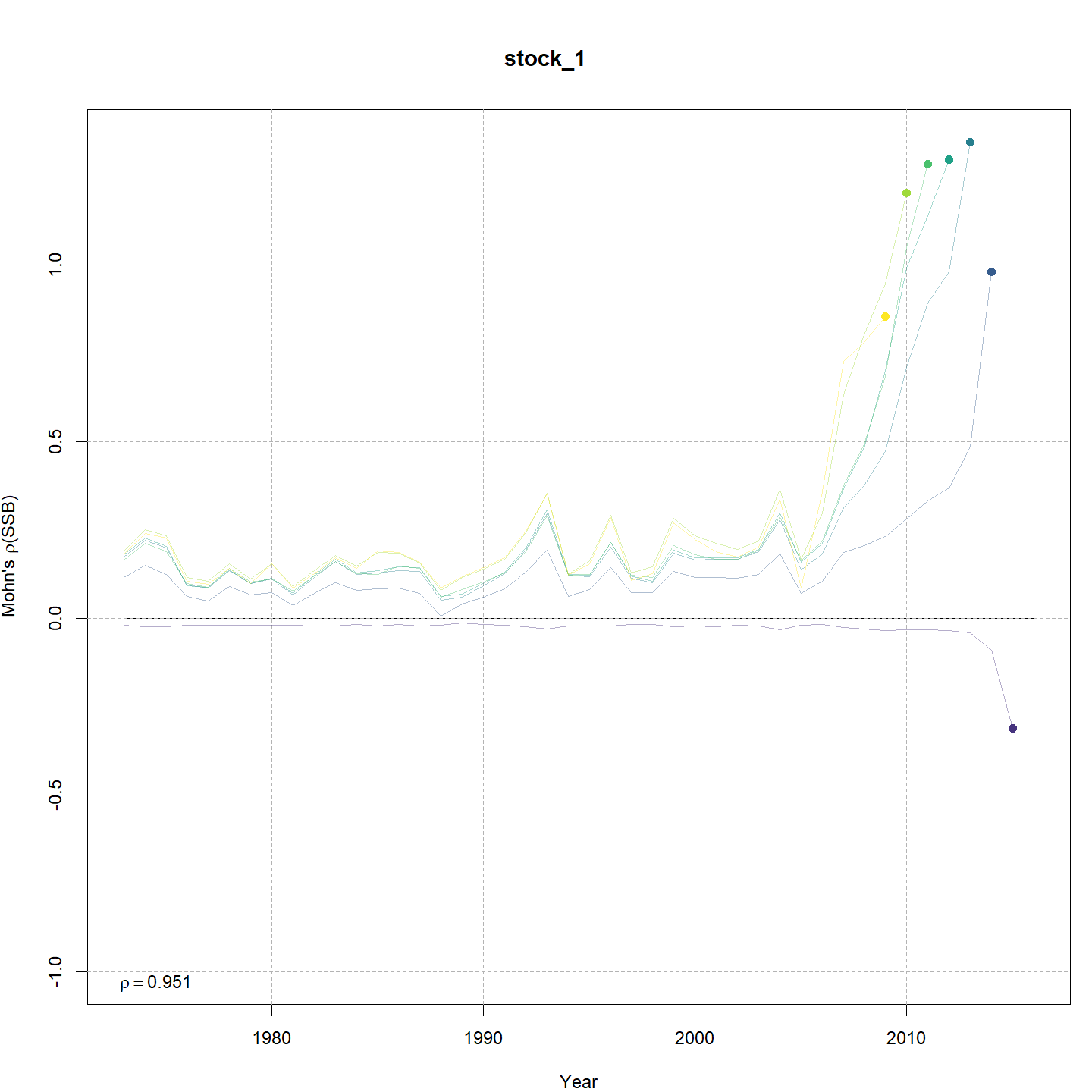
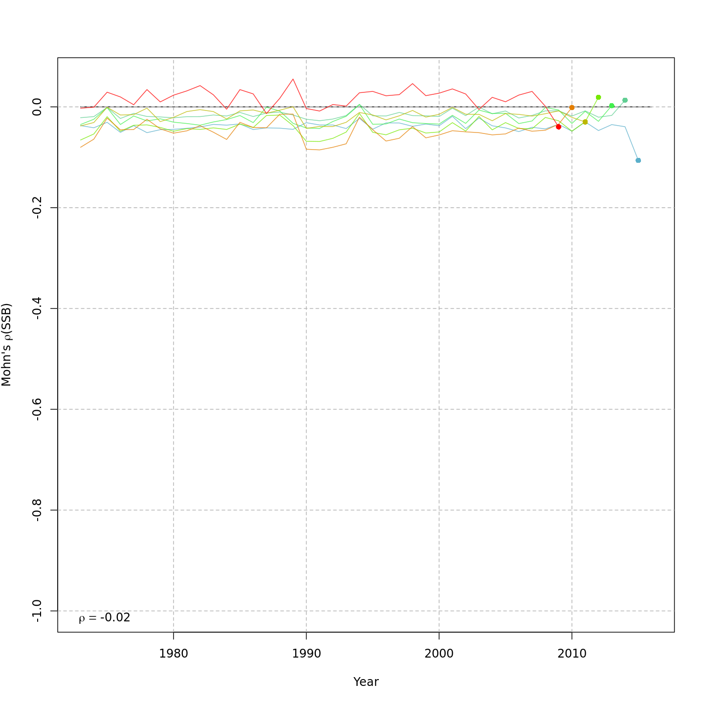
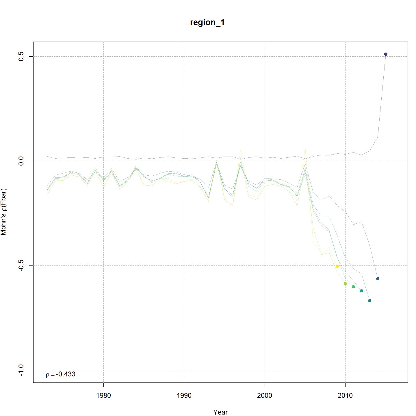
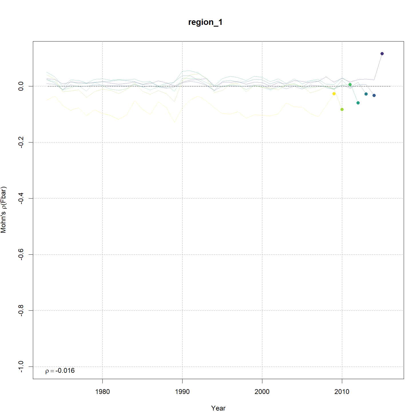
Retrospective patterns
The base model, m1 and all
NAA_re$sigma = "rec" models (m2-m3 and
m8-m9) had a severe retrospective pattern for recruitment,
SSB, and
(very high
).
The full state-space model effectively alleviated this. Adding a
GSI-Recruitment link to the state-space models further reduced
,
but had negligible effects on
and
.
The AIC and Mohn’s
values were similar for m11 and m13, the
models with lowest AIC.
The plots below compare retrospective patterns from the base model
(m1, left) to those from the full model (m13,
right).
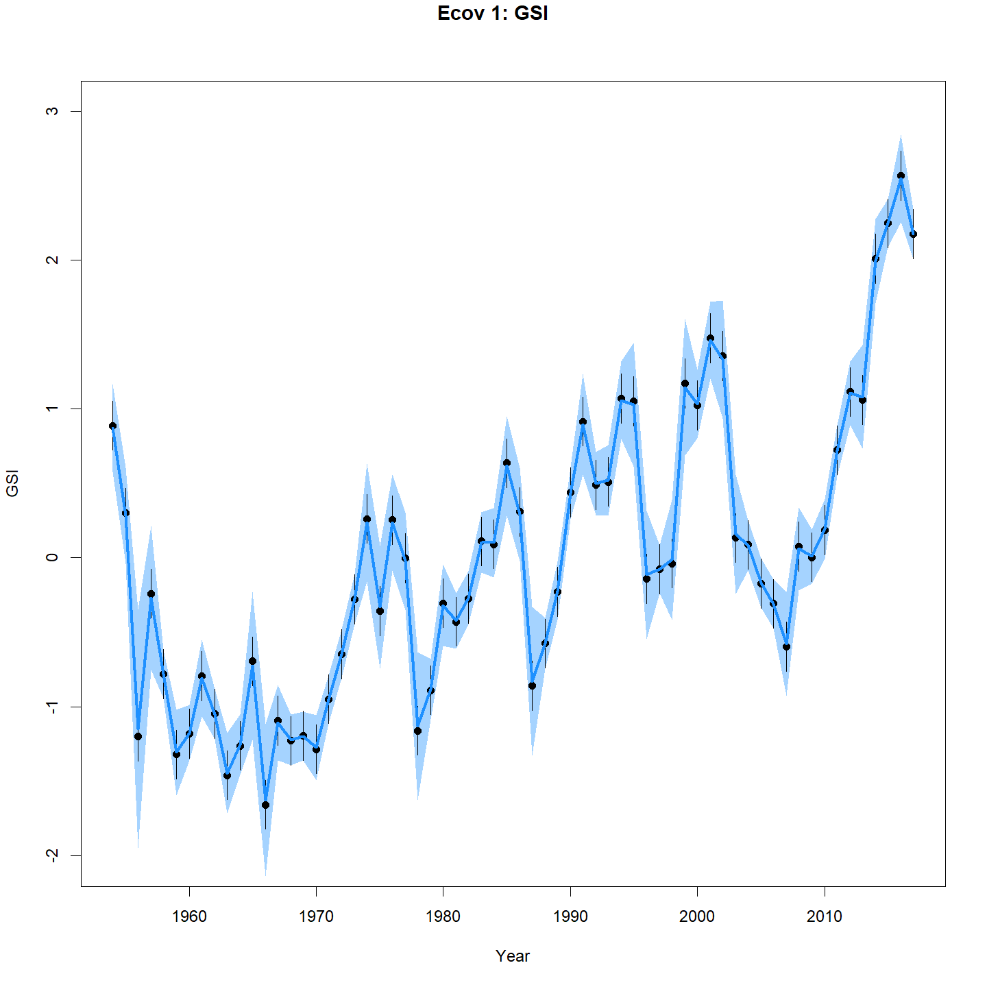
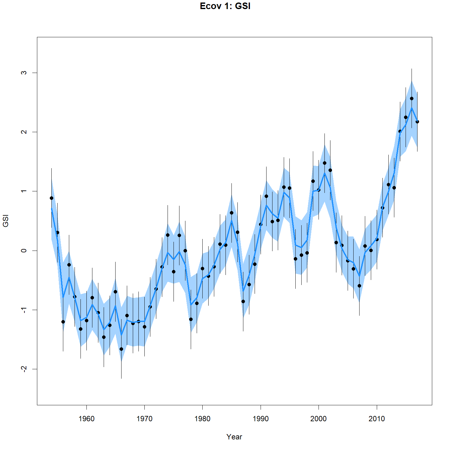
Estimated GSI
Models with a GSI-Recruitment link estimated higher observation error
and more smoothing of the GSI than those without. Compare the confidence
intervals for m7 (left, no GSI-Recruitment link), to those
for m13 (right, with GSI-Recruitment link).
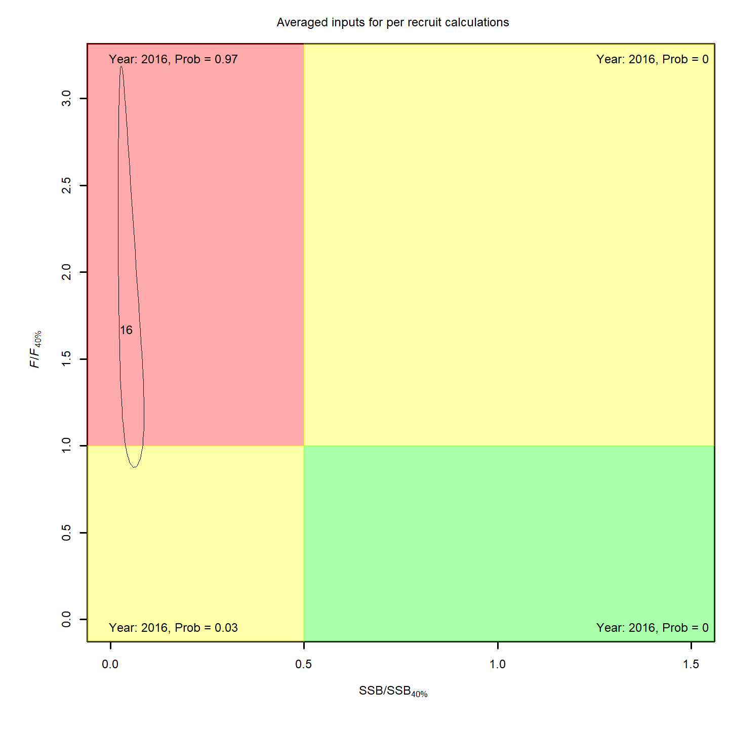
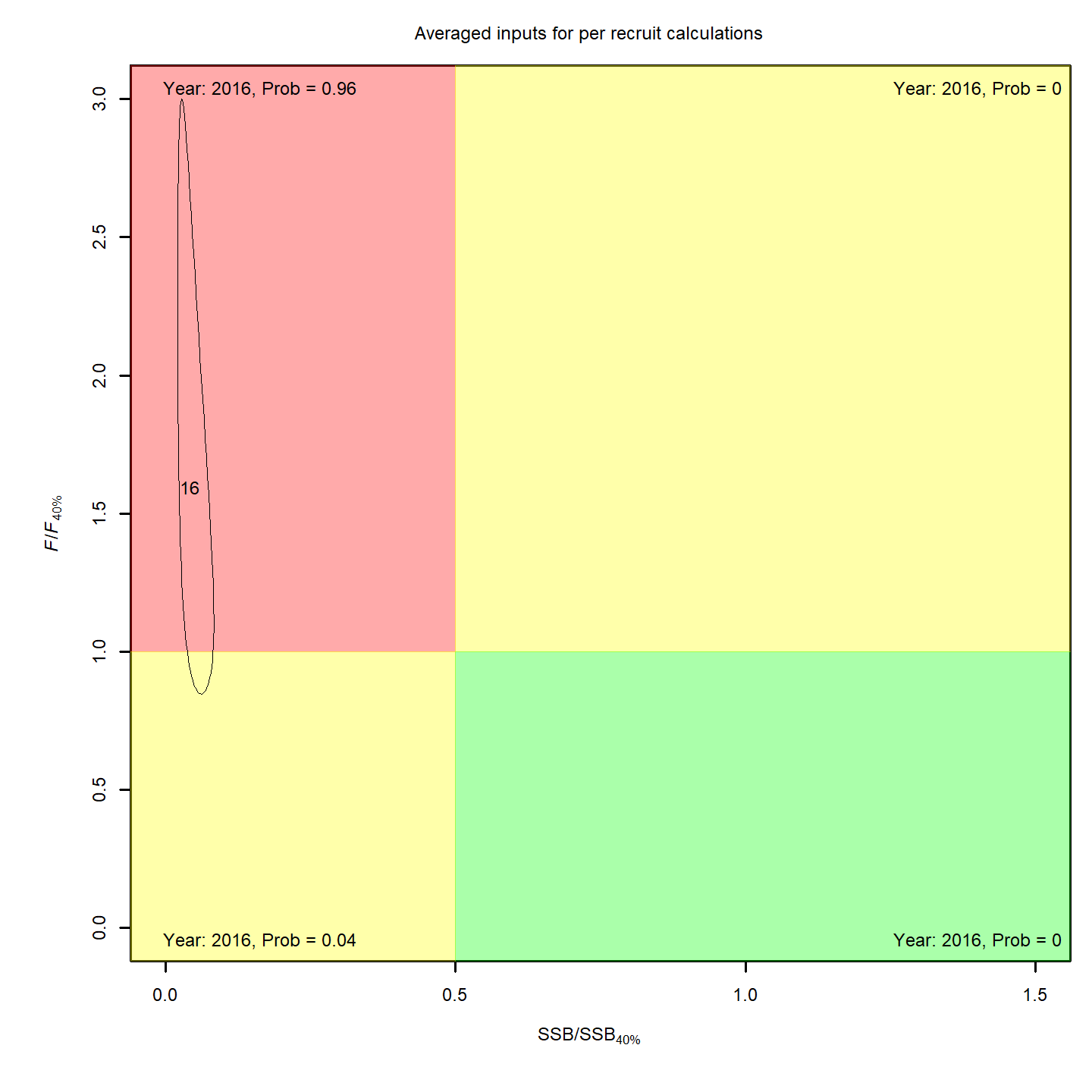
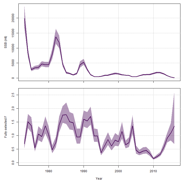
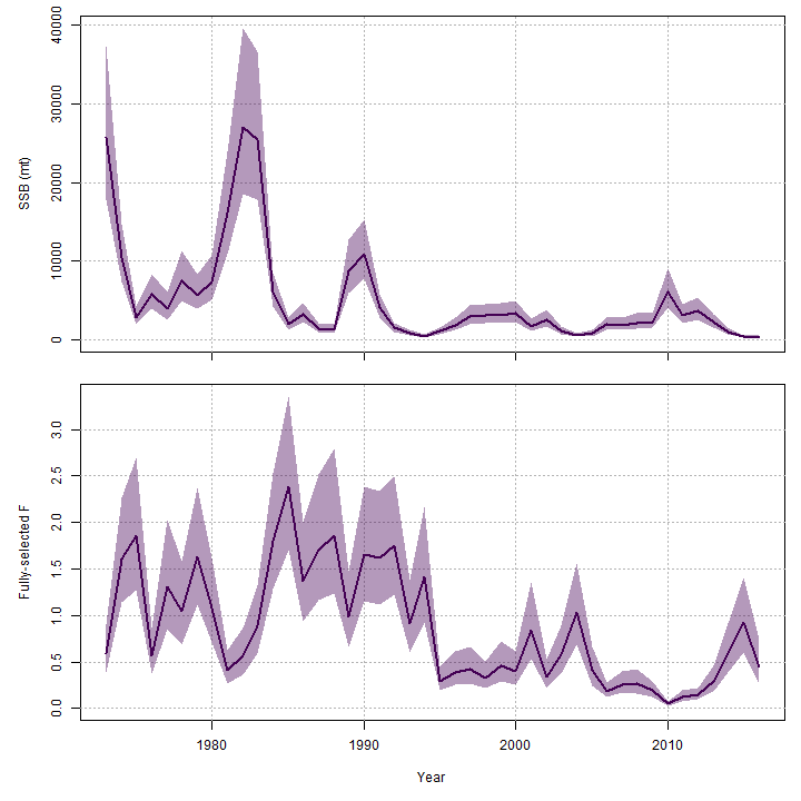
Stock status
The state-space models, with or without the GSI-Recruitment link,
estimated similar but slightly exaggerated trends in
and
compared to the base model. Left:
and
trends from the base model, m1. Right:
and
trends from the state-space model without GSI effect,
m7.
Adding the GSI-Recruitment link to the state-space model did not
impact the probability that the stock was overfished or experiencing
overfishing in the final year, 2016 (m7 w/o GSI, left;
m13 w/ GSI, right).