1. Background
This is the 11th WHAM example. We assume you already have
wham installed and are relatively familiar with the
package. If not, read the Introduction and Tutorial.
In this vignette we show how to both simulate and estimate:
- A prior distribution and random effect for catchability.
- Allow time-varying catchability as a random effect.
- Environmental covariate effect on catchability
- Different effects of the same environmental covariate on catchability and recruitment.
2. Setup
Create a directory for this analysis:
# choose a location to save output, otherwise will be saved in working directory
write.dir <- "choose/where/to/save/output"
dir.create(write.dir)
setwd(write.dir)
3. A simple operating model
Make a lists of information to pass to the basic_info ,
catch_info, index_info and F
arguments of prepare_wham_input. These components will
define a simple default stock and observations on it. We’ll then use the
input with fit_wham to create operating and estimating
models. This similar to example 10, but now there are two indices.
make_digifish <- function(years = 1975:2014) {
    digifish = list()
    digifish$ages <- 1:10
    digifish$years <- years
    digifish$n_fleets <- 1
    na = length(digifish$ages)
    ny = length(digifish$years)

    digifish$maturity = array(t(matrix(1/(1 + exp(-1*(1:na - na/2))), na, ny)), c(1,ny,na))

    L = 100*(1-exp(-0.3*(1:na - 0)))
    W = exp(-11)*L^3
    nwaa = 1
    digifish$waa = array(t(matrix(W, na, ny)), dim = c(1, ny, na))

    digifish$fracyr_SSB <- cbind(rep(0.25,ny))

    digifish$bias_correct_process <- TRUE
    digifish$bias_correct_observation <- TRUE
    return(digifish)
}
digifish = make_digifish()

catch_info <- list()
catch_info$n_fleets = 1
catch_info$catch_cv = matrix(0.1, length(digifish$years), digifish$n_fleets)
catch_info$catch_Neff = matrix(200, length(digifish$years), digifish$n_fleets)
catch_info$selblock_pointer_fleets = t(matrix(1:digifish$n_fleets, digifish$n_fleets, length(digifish$years)))
index_info <- list()
index_info$n_indices <- 2
index_info$index_cv = matrix(0.3, length(digifish$years), index_info$n_indices)
index_info$index_Neff = matrix(100, length(digifish$years), index_info$n_indices)
index_info$fracyr_indices = matrix(0.5, length(digifish$years), index_info$n_indices)
index_info$units_indices <- rep(2, index_info$n_indices) #abundance
index_info$units_index_paa <- rep(2, index_info$n_indices) #abundance
index_info$selblock_pointer_indices = t(matrix(digifish$n_fleets + 1:index_info$n_indices, index_info$n_indices, length(digifish$years)))
F_info <- list(F = matrix(0.2,length(digifish$years), catch_info$n_fleets))
Now define selectivity and M arguments for
prepare_wham_input.
selectivity = list(model = c(rep("logistic", digifish$n_fleets),rep("logistic", index_info$n_indices)),
    initial_pars = rep(list(c(5,1)), digifish$n_fleets + index_info$n_indices)) #fleet, index

M = list(initial_means = array(0.2, c(1,1,length(digifish$ages))))
Here we specify recruitment deviations are independent random effects and no stock-recruit relationship will be assumed.
NAA_re = list(
  N1_model = "age-specific-fe",
  N1_pars = array(exp(10)*exp(-(0:(length(digifish$ages)-1))*M$initial_means[1]), c(1,1,length(digifish$ages))))
NAA_re$sigma = "rec" #random about mean
#NAA_re$use_steepness = 0
NAA_re$recruit_model = 2 #random effects with a constant mean
NAA_re$recruit_pars = list(exp(10))
4. Setting up the q parameter for the second index to have a prior distribution.
We can use the initial_q and prior_sd
components of the catchability argument to specify a normal
prior distribution for logit catchability of one or more indices. The
lower and upper bounds of each catchability can be defined using
q_lower and q_upper elements of the
cactchability argument, but they are 0 and 1000 by default.
Entries in prior_sd that are NA do not have
time-varying random effects values and the corresponding value
initial_q will be the initial value when estimated or the
assumed catchability for simulation for an operating model. Non-NA
entries in prior_sd define the standard deviation of the
normal prior distribution and the corresponding value of
initial_q is the inverse-logit of the mean of the prior
distribution.
Now we can make the input list with
prepare_wham_input
input = suppressWarnings(prepare_wham_input(basic_info = digifish, selectivity = selectivity, NAA_re = NAA_re, M = M, catchability = catchability,
  index_info = index_info, catch_info = catch_info, F = F_info))
We can then define an operating model (OM) and simulate data as well as random effects for the q of the second survey and recruitment from this input. Note we first remove any parameters from the random component of the input so that TMB will not try to optimize these random effects if it would normallly when estimating a model. This is not necessary here, but it was for the closed-loop simulations in example 10, and would seem to be a good habit.
om_input <- input
om_input$random <- NULL
om = fit_wham(om_input, do.fit = FALSE, MakeADFun.silent = TRUE)

#simulate data from operating model
set.seed(0101010)
newdata = om$simulate(complete=TRUE)
Now put the simulated data in an input file with all the same configuration as the operating model.
temp = input
temp$data = newdata
Fit an estimation model that is the same as the operating model (self-test).
fit = fit_wham(temp, do.osa = FALSE, do.retro=FALSE, MakeADFun.silent = TRUE, retro.silent = TRUE)
plot_wham_output(fit)
This plot of the q prior and approximate posterior is provided by
plot_wham_output. The true simulated q is shown as the
solid vertical line.
wham:::plot_q_prior_post(fit)
abline(v = newdata$q[1,2], lwd = 2)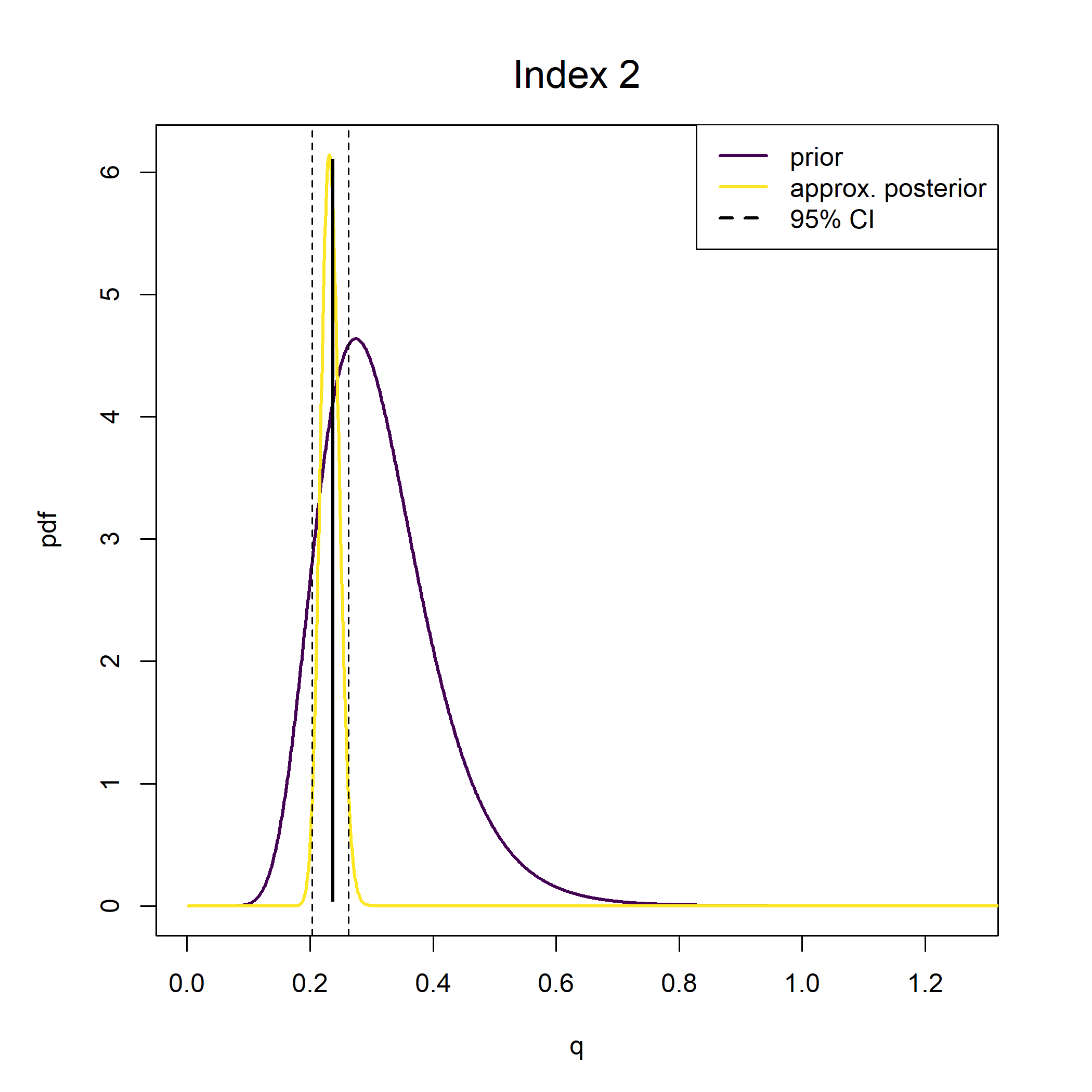
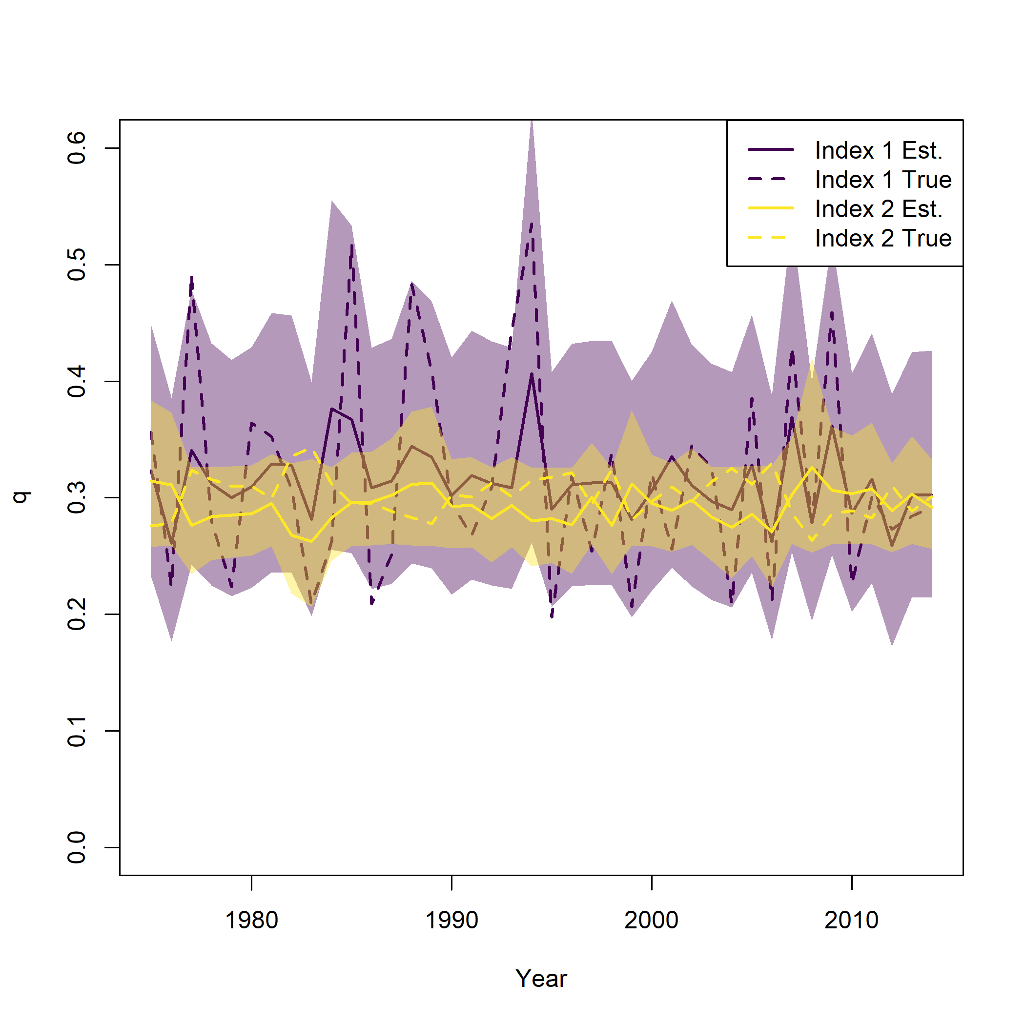
5. Add random effects on q for first index
This will add time varying iid random effects on catchability for the
first index while still keeping the prior on the second index. We
specify the standard deviation of the catchability of the random effects
on the logit scale with sigma_val.
catchability = list(prior_sd = c(NA, 0.3), initial_q = rep(0.3, index_info$n_indices), re = c("iid", "none"), sigma_val = c(0.3,0.3))Generate input as above.
input = prepare_wham_input(basic_info = digifish, selectivity = selectivity, NAA_re = NAA_re, M = M, catchability = catchability,
  index_info = index_info, catch_info = catch_info, F = F_info)
Now create the operating model, simulate data and fit as above
om_input <- input
om_input$random <- NULL
om = fit_wham(om_input, do.fit = FALSE, MakeADFun.silent = TRUE)

#simulate data from operating model
set.seed(0101010)
newdata = om$simulate(complete=TRUE)

#put the simulated data in an input file with all the same configuration as the operating model
temp = input
temp$data = newdata

#fit estimating model that is the same as the operating model
fit = fit_wham(temp, do.osa = FALSE, do.retro=FALSE, MakeADFun.silent = TRUE, retro.silent = TRUE)

plot_wham_output(fit)
This is similar to what is provided in plot_wham_output,
but with the true values from the simulation also plotted
pal = viridisLite::viridis(n=2)
plot(fit$years, fit$rep$q[,1], type = 'n', lwd = 2, col = pal[1], ylim = c(0,1), ylab = "q", xlab = "Year")
se = summary(fit$sdrep)
se = matrix(se[rownames(se) == "logit_q_mat",2], length(fit$years))
for( i in 1:input$data$n_indices){
  lines(fit$years, fit$rep$q[,i], lwd = 2, col = pal[i])
  polyy = c(fit$rep$q[,i]*exp(-1.96*se[,i]),rev(fit$rep$q[,i]*exp(1.96*se[,i])))
  polygon(c(fit$years,rev(fit$years)), polyy, col=adjustcolor(pal[i], alpha.f=0.4), border = "transparent")
  lines(fit$years, newdata$q[,i], lwd = 2, col = pal[i], lty = 2)
}
legend("topright", legend = paste0("Index ", rep(1:input$data$n_indices, each = 2), c(" Est.", " True")), lwd = 2, col = rep(pal, each = 2), lty = c(1,2))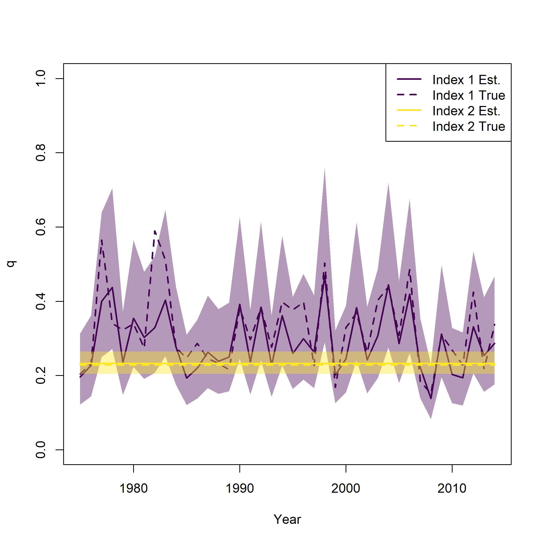
6. Add Environmental covariates to the model
First simulate and estimate environmental covariate processes, but no effects of population.
ecov = list(
        label = c("Climate variable 1", "Climate variable 2"),
        process_model = c("ar1","ar1"),
        mean = cbind(rnorm(length(digifish$years)),rnorm(length(digifish$years))),
        logsigma = log(c(0.01, 0.2)),
        years = digifish$years,
        use_obs = matrix(1,length(digifish$years),2),
        q_how = matrix("none",2,2))

ecov$process_mean_vals = c(0,0) #mean
ecov$process_sig_vals = c(0.1,0.2) #sd
ecov$process_cor_vals <- c(0.4,-0.3)  #cor
We use process_mean_vals, process_sig_vals
and process_cor_vals to specify parameters for the AR1
processes assumed for the environmental covariate processes. Note that
ecov$q_how is a matrix with rows for indices and columns
for covariates for whether each covariate affects an index. Note also,
that the simulated values for the observations for each covariate here
will not be used.
We will not include a prior distribution for the second index, but we will keep the iid random effects on q for the first index.
catchability = list(initial_q = rep(0.3, index_info$n_indices), sigma_val = c(0.3,0.3), re = c("iid", "none"))

input = prepare_wham_input(basic_info = digifish, selectivity = selectivity, NAA_re = NAA_re, M = M, catchability = catchability, ecov = ecov,
  index_info = index_info, catch_info = catch_info, F = F_info)
Now create the operating model and simulate and fit data.
om_input <- input
om_input$random <- NULL
om = fit_wham(om_input, do.fit = FALSE, MakeADFun.silent = TRUE)
set.seed(0101010)
newdata = om$simulate(complete=TRUE)

#put the simulated data in an input file with all the same configuration as the operating model
temp = input
temp$data = newdata

#fit estimating model that is the same as the operating model
fit = fit_wham(temp, do.osa = FALSE, do.retro = FALSE, MakeADFun.silent = TRUE)

plot_wham_output(fit)
Check the table of parameter estimates on the second tab of the html
document produced by plot_wham_output. It shows parameter
estiamtes, standard errors, and confidence intervals on the natural
scale of the parameters.
Again, this is similar to what is provided in
plot_wham_output, but with the true values from the
simulation also plotted.
pal = viridisLite::viridis(n=2)
se = summary(fit$sdrep)
se = matrix(se[rownames(se) == "logit_q_mat",2], length(fit$years))
plot(fit$years, fit$rep$q[,1], type = 'n', lwd = 2, col = pal[1], ylim = c(0,1), ylab = "q", xlab = "Year")
for( i in 1:input$data$n_indices){
    lines(fit$years, fit$rep$q[,i], lwd = 2, col = pal[i])
  polyy = c(fit$rep$q[,i]*exp(-1.96*se[,i]),rev(fit$rep$q[,i]*exp(1.96*se[,i])))
    polygon(c(fit$years,rev(fit$years)), polyy, col=adjustcolor(pal[i], alpha.f=0.4), border = "transparent")
    lines(fit$years, newdata$q[,i], lwd = 2, col = pal[i], lty = 2)
}
legend("topright", legend = paste0("Index ", rep(1:input$data$n_indices, each = 2), c(" Est.", " True")), lwd = 2, col = rep(pal, each = 2), lty = c(1,2))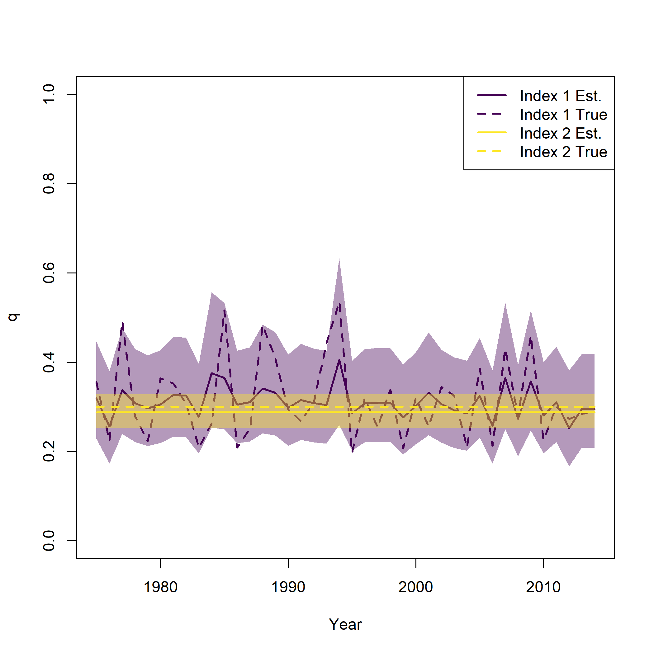
Let’s take a look at the true and estimated environmental covariate process pararameters. Columns are the different covariates. Rows are the mean, sd, and correlation parameters, respectively.
input$par$Ecov_process_pars
fit$parList$Ecov_process_pars
Compare true and estimated (log) standard deviation of time-varying q. First row, first column.
input$par$q_repars
fit$parList$q_repars
The estimated variability in q is lower than truth, but the estimate has large standard error:
as.list(fit$sdrep, "Std")$q_repars7. Environmental effects on catchability
Allow effects of first Environmental covariate on q for second index.
ecov$q_how <- matrix(c("none", "none","lag-0-linear","none"),2,2)

#set value for Ecov_beta effect on q (dims are n_effects (n_indices, n_Ecov, max_n_poly)
ecov$beta_q_vals <- array(0, dim = c(index_info$n_indices, length(ecov$label), 1))
ecov$beta_q_vals[2,1,1] <- 0.5
We set the value for effect of the environmental covariate on q using
ecov$beta_q_vals (array dims are n_indices, n_Ecov, order
of the polynomial).
As above, generate input.
input = prepare_wham_input(basic_info = digifish, selectivity = selectivity, NAA_re = NAA_re, M = M, catchability = catchability, ecov = ecov,
  index_info = index_info, catch_info = catch_info, F = F_info)
As above, create the operating model, simulate and fit data and compare true and estimated parameters.
om_input <- input
om_input$random <- NULL
om = fit_wham(om_input, do.fit = FALSE, MakeADFun.silent = TRUE)
set.seed(0101010)
newdata = om$simulate(complete=TRUE)

#put the simulated data in an input file with all the same configuration as the operating model
temp = input
temp$data = newdata

#fit estimating model that is the same as the operating model
fit = fit_wham(temp, do.osa = FALSE, do.retro = FALSE, MakeADFun.silent = TRUE)

plot_wham_output(fit)

#compare assumed and estimated ecov process pars
input$par$Ecov_beta[4,1,1,1]
fit$parList$Ecov_beta[4,1,1,1]

#compare assumed and estimated ecov process pars
input$par$Ecov_process_pars
fit$parList$Ecov_process_pars


#compare true and estimated time-varying q
input$par$q_repars
fit$parList$q_repars
#estimated variability in q is lower than truth, but estimate has large SE
as.list(fit$sdrep, "Std")$q_repars

pal = viridisLite::viridis(n=2)
se = summary(fit$sdrep)
se = matrix(se[rownames(se) == "logit_q_mat",2], length(fit$years))
plot(fit$years, fit$rep$q[,1], type = 'n', lwd = 2, col = pal[1], ylim = c(0,1), ylab = "q", xlab = "Year")
for( i in 1:input$data$n_indices){
    lines(fit$years, fit$rep$q[,i], lwd = 2, col = pal[i])
  polyy = c(fit$rep$q[,i]*exp(-1.96*se[,i]),rev(fit$rep$q[,i]*exp(1.96*se[,i])))
    polygon(c(fit$years,rev(fit$years)), polyy, col=adjustcolor(pal[i], alpha.f=0.4), border = "transparent")
    lines(fit$years, newdata$q[,i], lwd = 2, col = pal[i], lty = 2)
}
legend("topright", legend = paste0("Index ", rep(1:input$data$n_indices, each = 2), c(" Est.", " True")), lwd = 2, col = rep(pal, each = 2), lty = c(1,2))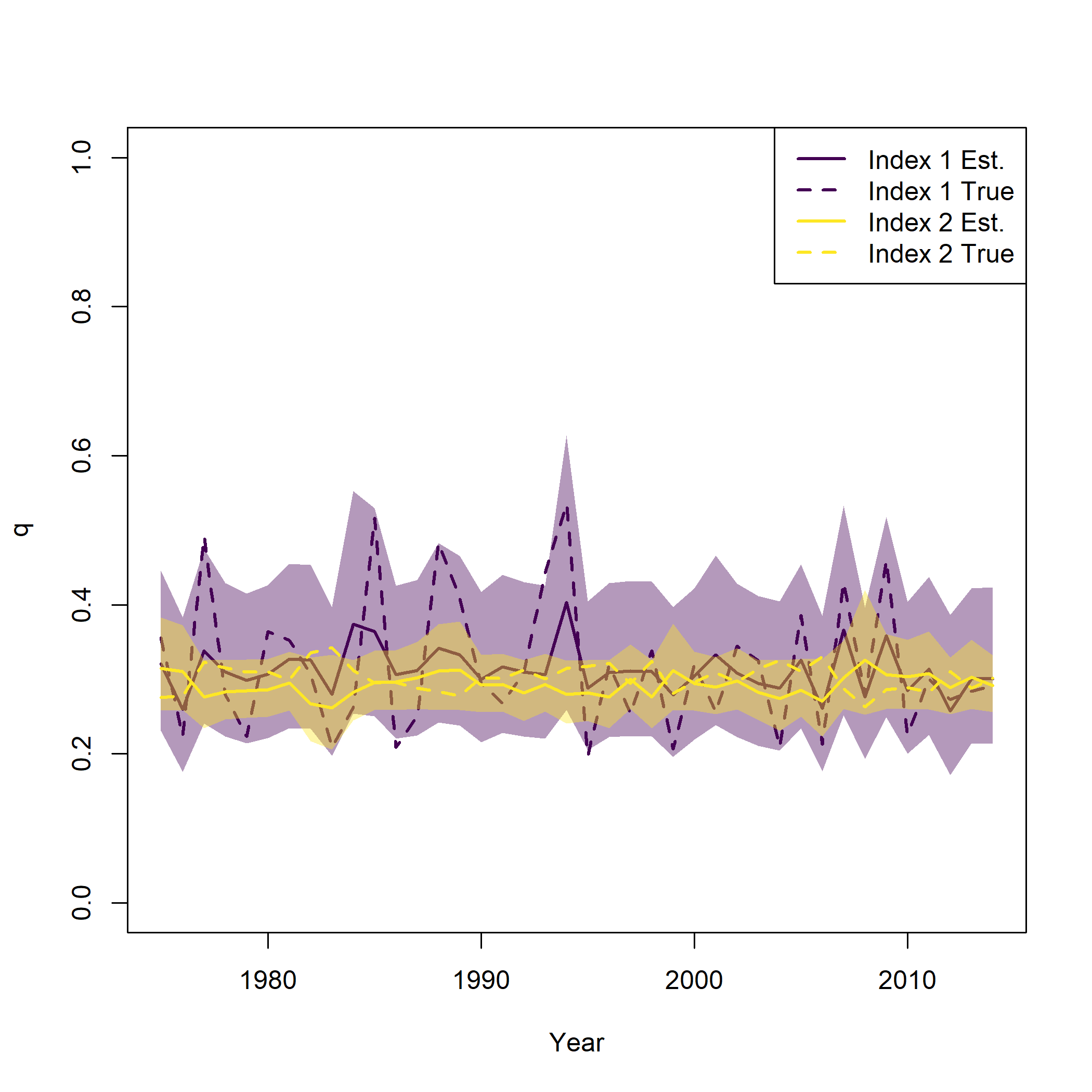
8. Different effects on q and recruitment of the same environmental covariate.
Add covariates to the model and allow effects of first covariate on q for second index AND recruitment. Then proceed as above. Use ecov$beta_R_vals to specify effect size of covariate on recruitment.
ecov$recruitment_how <- matrix(c("controlling-lag-0-linear","none"),2,1)

#set value for Ecov_beta effect on recruitment (dims are n_effects (2 + n_indices, max_n_poly, n_Ecov, n_ages)
ecov$beta_R_vals <- array(0, dim = c(1, length(ecov$label), 1))
ecov$beta_R_vals[1,1,1] <- -0.5

input = prepare_wham_input(basic_info = digifish, selectivity = selectivity, NAA_re = NAA_re, M = M, catchability = catchability, ecov = ecov,
  index_info = index_info, catch_info = catch_info, F = F_info)
Create the operating model, simulate and fit data, and compare true and estimated parameters.
om_input <- input
om_input$random <- NULL
om = fit_wham(om_input, do.fit = FALSE, MakeADFun.silent = TRUE)
set.seed(0101010)
newdata = om$simulate(complete=TRUE)

#put the simulated data in an input file with all the same configuration as the operating model
temp = input
temp$data = newdata

#fit estimating model that is the same as the operating model
fit = fit_wham(temp, do.osa = FALSE, do.retro = FALSE, MakeADFun.silent = TRUE)

plot_wham_output(fit)

#compare assumed and estimated ecov effect on q for second index
input$par$Ecov_beta_q[2,1,1]
fit$parList$Ecov_beta_q[2,1,1]

#compare assumed and estimated ecov effect on recruitment
input$par$Ecov_beta_R[1,1,1]
fit$parList$Ecov_beta_R[1,1,1]

#SE for beta parameters is large, especially for recruitment effect
as.list(fit$sdrep, "Std")$Ecov_beta_q[2,1,1]
as.list(fit$sdrep, "Std")$Ecov_beta_R[1,1,1]

#compare assumed and estimated ecov process pars
input$par$Ecov_process_pars
fit$parList$Ecov_process_pars

#compare true and estimated time-varying q
input$par$q_repars
fit$parList$q_repars

#estimated variability in q is lower than truth, but estimate has large SE
as.list(fit$sdrep, "Std")$q_repars

pal = viridisLite::viridis(n=2)
se = summary(fit$sdrep)
se = matrix(se[rownames(se) == "logit_q_mat",2], length(fit$years))
plot(fit$years, fit$rep$q[,1], type = 'n', lwd = 2, col = pal[1], ylim = c(0,0.6), ylab = "q", xlab = "Year")
for( i in 1:input$data$n_indices){
    lines(fit$years, fit$rep$q[,i], lwd = 2, col = pal[i])
  polyy = c(fit$rep$q[,i]*exp(-1.96*se[,i]),rev(fit$rep$q[,i]*exp(1.96*se[,i])))
    polygon(c(fit$years,rev(fit$years)), polyy, col=adjustcolor(pal[i], alpha.f=0.4), border = "transparent")
    lines(fit$years, newdata$q[,i], lwd = 2, col = pal[i], lty = 2)
}
legend("topright", legend = paste0("Index ", rep(1:input$data$n_indices, each = 2), c(" Est.", " True")), lwd = 2, col = rep(pal, each = 2), lty = c(1,2))