Ex 5: Time-varying natural mortality linked to the Gulf Stream Index • wham

In this vignette we walk through an example using the wham (WHAM = Woods Hole Assessment Model) package to run a state-space age-structured stock assessment model. WHAM is a generalization of code written for Miller et al. (2016) and Xu et al. (2018), and in this example we apply WHAM to the same stock, Southern New England / Mid-Atlantic Yellowtail Flounder.

This is the 5th WHAM example, which builds off example 2:

full state-space model (numbers-at-age are random effects for all ages, NAA_re = list(sigma='rec+1',cor='iid'))
logistic normal age compositions, pooling zero observations with adjacent ages (age_comp = "logistic-normal-pool0")
random-about-mean recruitment (recruit_model = 2)
5 indices
fit to 1973-2011 data

We assume you already have wham installed. If not, see the Introduction. The simpler 1st example, without environmental effects or time-varying $M$, is available as a R script and vignette.

In example 5, we demonstrate how to specify and run WHAM with the following options for natural mortality:

not estimated (fixed at input values)
one value, $M$
age-specific, $M_a$ (independent)
function of weight-at-age, $M_{y,a} = \mu_M * W_{y,a}^b$
AR1 deviations by age (random effects), $M_{y,a} = \mu_M + \delta_a \quad\mathrm{and}\quad \delta_a \sim \mathcal{N} (\rho_a \delta_{a-1}, \sigma^2_M)$
AR1 deviations by year (random effects), $M_{y,a} = \mu_M + \delta_y \quad\mathrm{and}\quad \delta_y \sim \mathcal{N} (\rho_y \delta_{y-1}, \sigma^2_M)$
2D AR1 deviations by age and year (random effects), $M_{y,a} = M_a + \delta_{y,a} \quad\mathrm{and}\quad \delta_{y,a} \sim \mathcal{N}(0,\Sigma)$

We also demonstrate alternate specifications for the link between $M$ and an environmental covariate, the Gulf Stream Index (GSI), as in O’Leary et al. (2019):

none
linear (in log-space), $M_{y,a} = e^{\mathrm{log}\mu_M + \beta_1 E_y}$
quadratic (in log-space), $M_{y,a} = e^{\mathrm{log}\mu_M + \beta_1 E_y + \beta_2 E^2_y}$

Note that you can specify more than one of the above effects on $M$, although the model may not be estimable. For example, the most complex model with weight-at-age, 2D AR1 age- and year-deviations, and a quadratic environmental effect: $M_{y,a} = e^{\mathrm{log}\mu_M + b W_{y,a} + \beta_1 E_y + \beta_2 E^2_y + \delta_{y,a}}$.

1. Load data

Open R and load the wham package:

library(wham)
library(tidyverse)
library(viridis)

For a clean, runnable .R script, look at ex5_M_GSI.R in the example_scripts folder of the wham package install:

wham.dir <- find.package("wham")
file.path(wham.dir, "example_scripts")

You can run this entire example script with:

write.dir <- "choose/where/to/save/output" # otherwise will be saved in working directory
source(file.path(wham.dir, "example_scripts", "ex5_M_GSI.R"))

Let’s create a directory for this analysis:

# choose a location to save output, otherwise will be saved in working directory
write.dir <- "choose/where/to/save/output"
dir.create(write.dir)
setwd(write.dir)

We need the same ASAP data file as in example 2, and the environmental covariate (GSI). Let’s copy ex2_SNEMAYT.dat and GSI.csv to our analysis directory:

wham.dir <- find.package("wham")
file.copy(from=file.path(wham.dir,"extdata","ex2_SNEMAYT.dat"), to=write.dir, overwrite=FALSE)
file.copy(from=file.path(wham.dir,"extdata","GSI.csv"), to=write.dir, overwrite=FALSE)

Confirm you are in the correct directory and it has the required data files:

list.files()

Read the ASAP3 .dat file into R and convert to input list for wham:

asap3 <- read_asap3_dat("ex2_SNEMAYT.dat")

Load the environmental covariate (Gulf Stream Index, GSI) data into R:

env.dat <- read.csv("GSI.csv", header=T)
head(env.dat)
#>   year        GSI
#> 1 1954  0.8876748
#> 2 1955  0.3024170
#> 3 1956 -1.2004947
#> 4 1957 -0.2408031
#> 5 1958 -0.7806940
#> 6 1959 -1.3218938

The GSI does not have a standard error estimate, either for each yearly observation or one overall value. In such a case, WHAM can estimate the observation error for the environmental covariate, either as one overall value, $\sigma_E$, or yearly values as random effects, $\mathrm{log}\sigma_{E_y} \sim \mathcal{N}(\mathrm{log}\sigma_E, \sigma^2_{\sigma_E})$. In this example we choose the simpler option and estimate one observation error parameter, shared across years.

2. Specify models

Now we specify several models with different options for natural mortality:

df.mods <- data.frame(M_model = c(rep("---",3),"age-specific","weight-at-age",rep("constant",5),"---"),
                      M_re = c(rep("none",6),"ar1_y","2dar1","none","none","2dar1"),
                      Ecov_process = rep("ar1",11),
                      Ecov_link = c(0,1,2,rep(0,5),1,2,0), stringsAsFactors=FALSE)
n.mods <- dim(df.mods)[1]
df.mods$Model <- paste0("m",1:n.mods)
df.mods <- df.mods %>% select(Model, everything()) # moves Model to first col

Look at the model table:

df.mods
#>    Model       M_model  M_re Ecov_process Ecov_link
#> 1     m1           ---  none          ar1         0
#> 2     m2           ---  none          ar1         1
#> 3     m3           ---  none          ar1         2
#> 4     m4  age-specific  none          ar1         0
#> 5     m5 weight-at-age  none          ar1         0
#> 6     m6      constant  none          ar1         0
#> 7     m7      constant ar1_y          ar1         0
#> 8     m8      constant 2dar1          ar1         0
#> 9     m9      constant  none          ar1         1
#> 10   m10      constant  none          ar1         2
#> 11   m11           --- 2dar1          ar1         0

3. Natural mortality options

Next we specify the options for modeling natural mortality by including an optional list argument, M, to the prepare_wham_input() function (see the prepare_wham_input() help page). M specifies estimation options and can overwrite M-at-age values specified in the ASAP data file. By default (i.e. M is NULL or not included), the M-at-age matrix from the ASAP data file is used (M fixed, not estimated). M is a list with the following entries:

$model: Natural mortality model options.
- "constant": estimate a single $M$, shared across all ages and years.
- "age-specific": estimate $M_a$ independent for each age, shared across years.
- "weight-at-age": estimate $M$ as a function of weight-at-age, $M_{y,a} = \mu_M * W_{y,a}^b$, as in Lorenzen (1996) and Miller & Hyun (2018).
$re: Time- and age-varying random effects on $M$.
- "none": $M$ constant in time and across ages (default).
- "iid": $M$ varies by year and age, but uncorrelated.
- "ar1_a": $M$ correlated by age (AR1), constant in time.
- "ar1_y": $M$ correlated by year (AR1), constant by age.
- "2dar1": $M$ correlated by year and age (2D AR1), as in Cadigan (2016).
$initial_means: Initial/mean M-at-age vector, with length = number of ages (if $model = "age-specific") or 1 (if $model = "weight-at-age" or "constant"). If NULL, initial mean M-at-age values are taken from the first row of the MAA matrix in the ASAP data file.
$est_ages: Vector of ages to estimate age-specific $M_a$ (others will be fixed at initial values). E.g. in a model with 6 ages, $est_ages = 5:6 will estimate $M_a$ for the 5th and 6th ages, and fix $M$ for ages 1-4. If NULL, $M$ at all ages is fixed at M$initial_means (if not NULL) or row 1 of the MAA matrix from the ASAP file (if M$initial_means = NULL).
$logb_prior: (Only for weight-at-age model) TRUE or FALSE (default), should a $\mathcal{N}(0.305, 0.08)$ prior be used on log_b? Based on Fig. 1 and Table 1 (marine fish) in Lorenzen (1996).

For example, to fit model m1, fix $M_a$ at values in ASAP file:

M <- NULL # or simply leave out of call to prepare_wham_input

To fit model m6, estimate one $M$, constant by year and age:

M <- list(model="constant", est_ages=1)

And to fit model m8, estimate mean $M$ with 2D AR1 deviations by year and age:

M <- list(model="constant", est_ages=1, re="2dar1")

To fit model m11, use the $M_a$ values specified in the ASAP file, but with 2D AR1 deviations as in Cadigan (2016):

M <- list(re="2dar1")

4. Linking M to an environmental covariate (GSI)

As described in example 2, the environmental covariate options are fed to prepare_wham_input() as a list, ecov. This example differs from example 2 in that:

$logsigma = "est_1": estimate the observation error for the GSI (one overall value for all years). The other option is "est_re" to allow the GSI observation error to have yearly fluctuations (random effects). The Cold Pool Index in example 2 had yearly observation errors given.
$lag = 0: GSI in year t affects $M$ in year t, instead of year t+1.
$where = "M": GSI affects $M$, instead of recruitment.
$how: ecov$how = 0 estimates the GSI time-series model (AR1) for models without a GSI-M effect, in order to compare AIC with models that do include a GSI-M effect. Setting ecov$how = 1 is necessary to allow a GSI-M effect.
$link_model: specifies the model linking GSI to $M$. Can be NA (no effect, default), "linear", or "poly-x" (where x is the degree of a polynomial). In this example we demonstrate models with no GSI-M effect, a linear GSI-M effect, and a quadratic GSI-M effect ("poly-2"). WHAM includes a function to calculate orthogonal polynomials in TMB, akin to the poly() function in R.

For example, the ecov list for model m3 with a quadratic GSI-M effect:

  # example for model m3
  ecov <- list(
    label = "GSI",
    mean = as.matrix(env.dat$GSI),
    logsigma = 'est_1', # estimate obs sigma, 1 value shared across years
    year = env.dat$year,
    use_obs = matrix(1, ncol=1, nrow=dim(env.dat)[1]), # use all obs (=1)
    lag = 0, # GSI in year t affects M in same year
    process_model = "ar1", # GSI modeled as AR1 (random walk would be "rw")
    where = "M", # GSI affects natural mortality
    how = 1, # include GSI effect on M
    link_model = "poly-2") # quadratic GSI-M effect

Note that you can set ecov = NULL to fit the model without environmental covariate data, but here we fit the ecov data even for models without GSI effect on $M$ (m1, m4-8) so that we can compare them via AIC (need to have the same data in the likelihood). We accomplish this by setting ecov$how = 0 and ecov$process_model = "ar1".

5. Run all models

All models use the same options for recruitment (random-about-mean, no stock-recruit function) and selectivity (logistic, with parameters fixed for indices 4 and 5).

env.dat <- read.csv("GSI.csv", header=T)
for(m in 1:n.mods){
  ecov <- list(
    label = "GSI",
    mean = as.matrix(env.dat$GSI),
    logsigma = 'est_1', # estimate obs sigma, 1 value shared across years
    year = env.dat$year,
    use_obs = matrix(1, ncol=1, nrow=dim(env.dat)[1]), # use all obs (=1)
    lag = 0, # GSI in year t affects M in same year
    process_model = df.mods$Ecov_process[m], # "rw" or "ar1"
    where = "M", # GSI affects natural mortality
    how = ifelse(df.mods$Ecov_link[m]==0,0,1), # 0 = no effect (but still fit Ecov to compare AIC), 1 = mean
    link_model = c(NA,"linear","poly-2")[df.mods$Ecov_link[m]+1])

  m_model <- df.mods$M_model[m]
  if(df.mods$M_model[m] == '---') m_model = "age-specific"
  if(df.mods$M_model[m] %in% c("constant","weight-at-age")) est_ages = 1
  if(df.mods$M_model[m] == "age-specific") est_ages = 1:asap3$dat$n_ages
  if(df.mods$M_model[m] == '---') est_ages = NULL
  
  M <- list(
    model = m_model,
    re = df.mods$M_re[m],
    est_ages = est_ages
  )
  if(m_model %in% c("constant","weight-at-age")) M$initial_means = 0.28

  input <- prepare_wham_input(asap3, recruit_model = 2,
                              model_name = paste0("m",m,": ", df.mods$M_model[m]," + ",c("no","linear","poly-2")[df.mods$Ecov_link[m]+1]," GSI link + ",df.mods$M_re[m]," devs"),
                              ecov = ecov,
                              selectivity=list(model=rep("logistic",6),
                                               initial_pars=c(rep(list(c(3,3)),4), list(c(1.5,0.1), c(1.5,0.1))),
                                               fix_pars=c(rep(list(NULL),4), list(1:2, 1:2))),
                              NAA_re = list(sigma='rec+1',cor='iid'),
                              M=M,
                              age_comp = "logistic-normal-pool0") # logistic normal pool 0 obs

  # Fit model
  mod <- fit_wham(input, do.retro=T, do.osa=F) # turn off OSA residuals to save time

  # Save model
  saveRDS(mod, file=paste0(df.mods$Model[m],".rds"))

  # If desired, plot output in new subfolder
  # plot_wham_output(mod=mod, dir.main=file.path(getwd(),df.mods$Model[m]), out.type='html')
  
  # If desired, do projections
  # mod_proj <- project_wham(mod)
  # saveRDS(mod_proj, file=paste0(df.mods$Model[m],"_proj.rds"))
}

6. Compare models

Collect all models into a list.

mod.list <- paste0(df.mods$Model,".rds")
mods <- lapply(mod.list, readRDS)

Get model convergence and stats.

opt_conv = 1-sapply(mods, function(x) x$opt$convergence)
ok_sdrep = sapply(mods, function(x) if(x$na_sdrep==FALSE & !is.na(x$na_sdrep)) 1 else 0)
df.mods$conv <- as.logical(opt_conv)
df.mods$pdHess <- as.logical(ok_sdrep)

Only calculate AIC and Mohn’s rho for converged models.

df.mods$runtime <- sapply(mods, function(x) x$runtime)
df.mods$NLL <- sapply(mods, function(x) round(x$opt$objective,3))
not_conv <- !df.mods$conv | !df.mods$pdHess
mods2 <- mods
mods2[not_conv] <- NULL
df.aic.tmp <- as.data.frame(compare_wham_models(mods2, sort=FALSE, calc.rho=T)$tab)
df.aic <- df.aic.tmp[FALSE,]
ct = 1
for(i in 1:n.mods){
  if(not_conv[i]){
    df.aic[i,] <- rep(NA,5)
  } else {
    df.aic[i,] <- df.aic.tmp[ct,]
    ct <- ct + 1
  }
}
df.aic[,1:2] <- format(round(df.aic[,1:2], 1), nsmall=1)
df.aic[,3:5] <- format(round(df.aic[,3:5], 3), nsmall=3)
df.aic[grep("NA",df.aic$dAIC),] <- "---"
df.mods <- cbind(df.mods, df.aic)

Make results table prettier.

df.mods$Ecov_link <- c("---","linear","poly-2")[df.mods$Ecov_link+1]
df.mods$M_re[df.mods$M_re=="none"] = "---"
colnames(df.mods)[2] = "M_est"
rownames(df.mods) <- NULL

Look at results table.

df.mods

7. Results

In the table, I have highlighted models which converged and successfully inverted the Hessian to produce SE estimates for all (fixed effect) parameters. WHAM stores this information in mod$na_sdrep (should be FALSE), mod$sdrep$pdHess (should be TRUE), and mod$opt$convergence (should be 0). See stats::nlminb() and TMB::sdreport() for details.

Models m8 (estimate mean $M$ and 2D AR1 deviations by year and age, no GSI effect) and m11 (keep mean $M$ fixed but estimate 2D AR1 deviations) had the lowest AIC and were overwhelmingly supported relative to the other models (bold in table below).

Model	M model	M_re	GSI	GSI link	Converged	Pos def Hessian	Runtime (min)	NLL	dAIC	AIC	$\rho_{R}$	$\rho_{SSB}$	$\rho_{\overline{F}}$
m1	—	—	ar1	—	TRUE	TRUE	0.19	-819.662	27.4	-1501.3	0.231	0.071	-0.111
m2	—	—	ar1	linear	TRUE	TRUE	0.25	-824.396	19.9	-1508.8	0.299	0.096	-0.127
m3	—	—	ar1	poly-2	TRUE	TRUE	2.95	-824.781	21.1	-1507.6	0.334	0.113	-0.135
m4	age-specific	—	ar1	—	TRUE	FALSE	0.21	-838.807	—	—	—	—	—
m5	weight-at-age	—	ar1	—	TRUE	TRUE	0.20	-826.112	18.5	-1510.2	0.679	0.133	-0.140
m6	constant	—	ar1	—	TRUE	TRUE	0.19	-826.106	16.5	-1512.2	0.509	0.123	-0.137
m7	constant	ar1_y	ar1	—	TRUE	TRUE	0.25	-826.521	19.7	-1509.0	1.182	0.433	-0.306
m8	constant	2dar1	ar1	—	TRUE	TRUE	0.92	-837.360	0.0	-1528.7	0.322	0.013	-0.051
m9	constant	—	ar1	linear	TRUE	TRUE	0.28	-830.636	9.4	-1519.3	0.293	0.033	-0.077
m10	constant	—	ar1	poly-2	TRUE	TRUE	2.93	-830.678	11.3	-1517.4	0.297	0.037	-0.080
m11	—	2dar1	ar1	—	TRUE	TRUE	0.98	-835.676	1.3	-1527.4	0.037	-0.045	0.022

Estimated M

Models allowed to estimate mean $M$ increased $M$ compared to the fixed values in m1-3 (more green/yellow than blue).
Models that estimated $M_a$ had highest $M_a$ for ages 4-5.
Models that estimated $M_y$ had higher $M_y$ in the early 1990s and around 2000.

Below is a plot of $M$ by age (y-axis) and year (x-axis) for all models. Models with a positive definite Hessian are solid, and models with non-positive definite Hessian are pale.

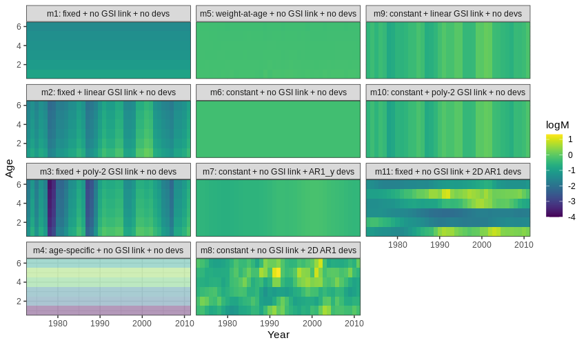
Natural mortality by age (y-axis) and year (x-axis) for all models.

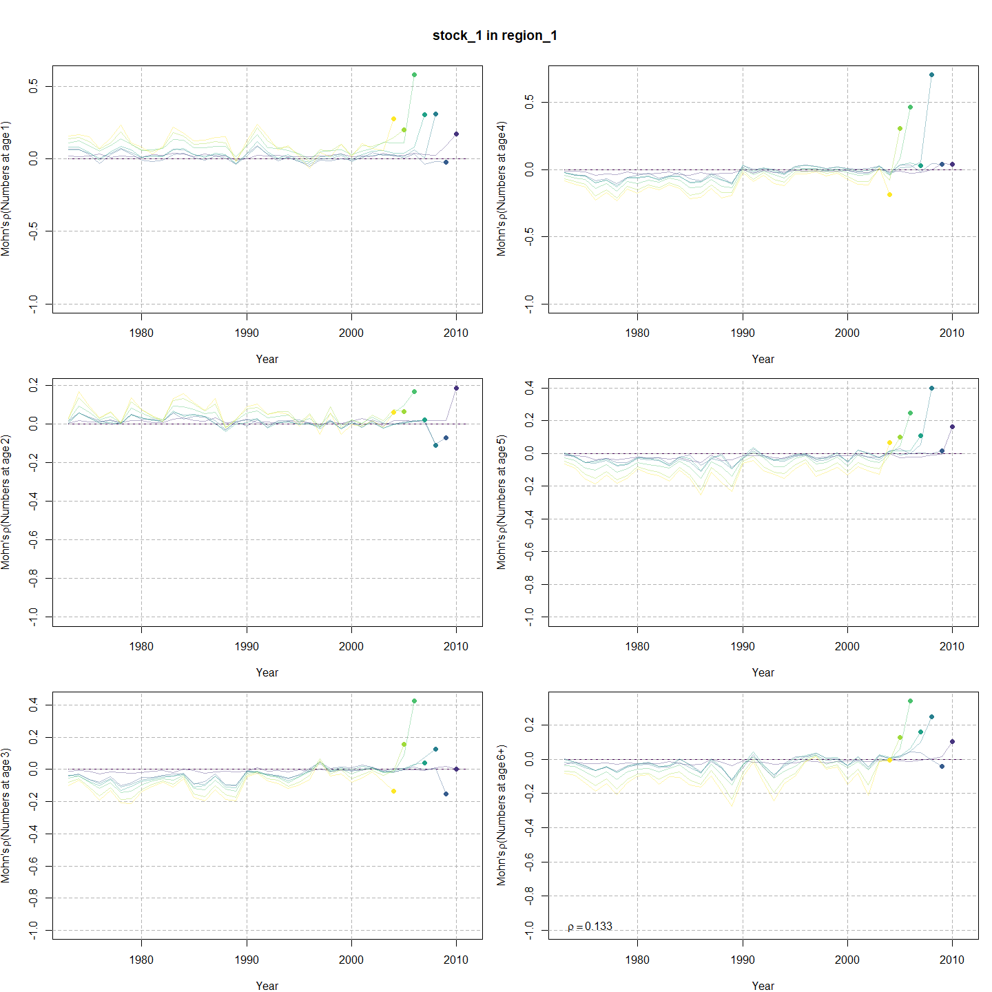
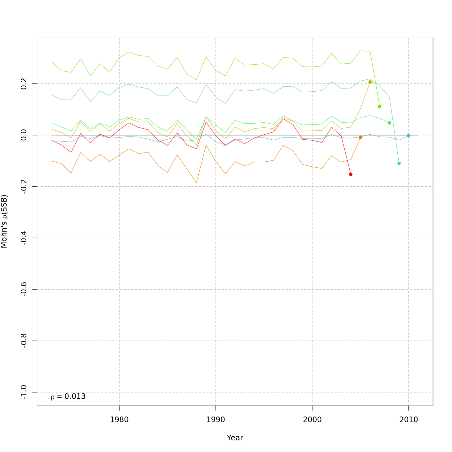
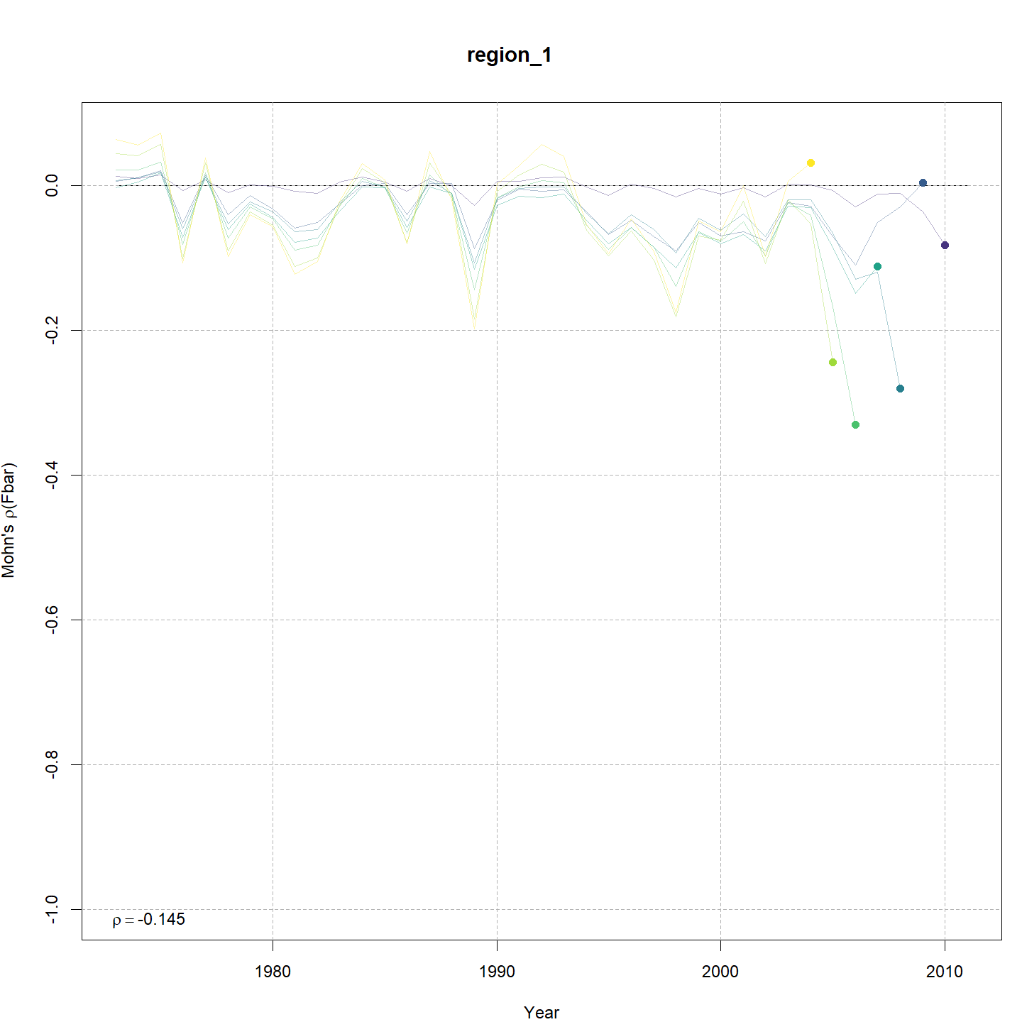
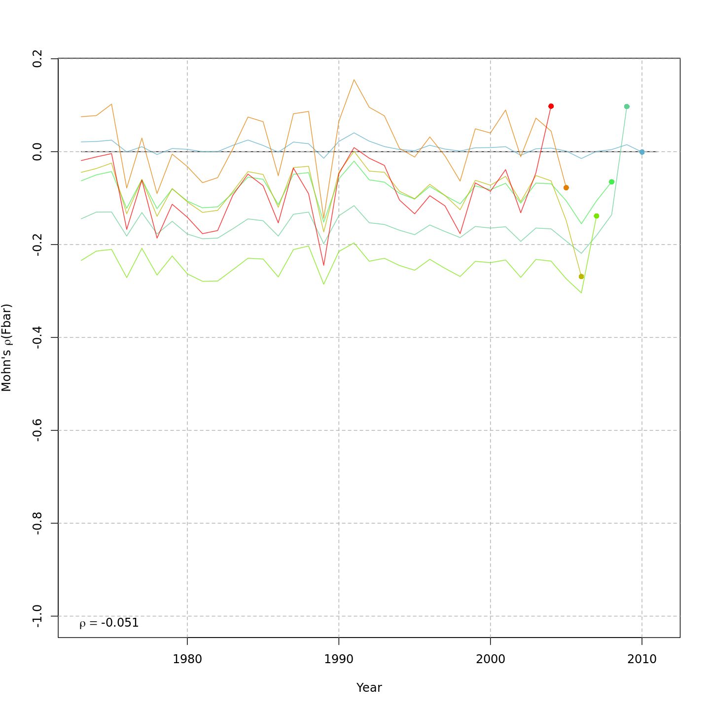
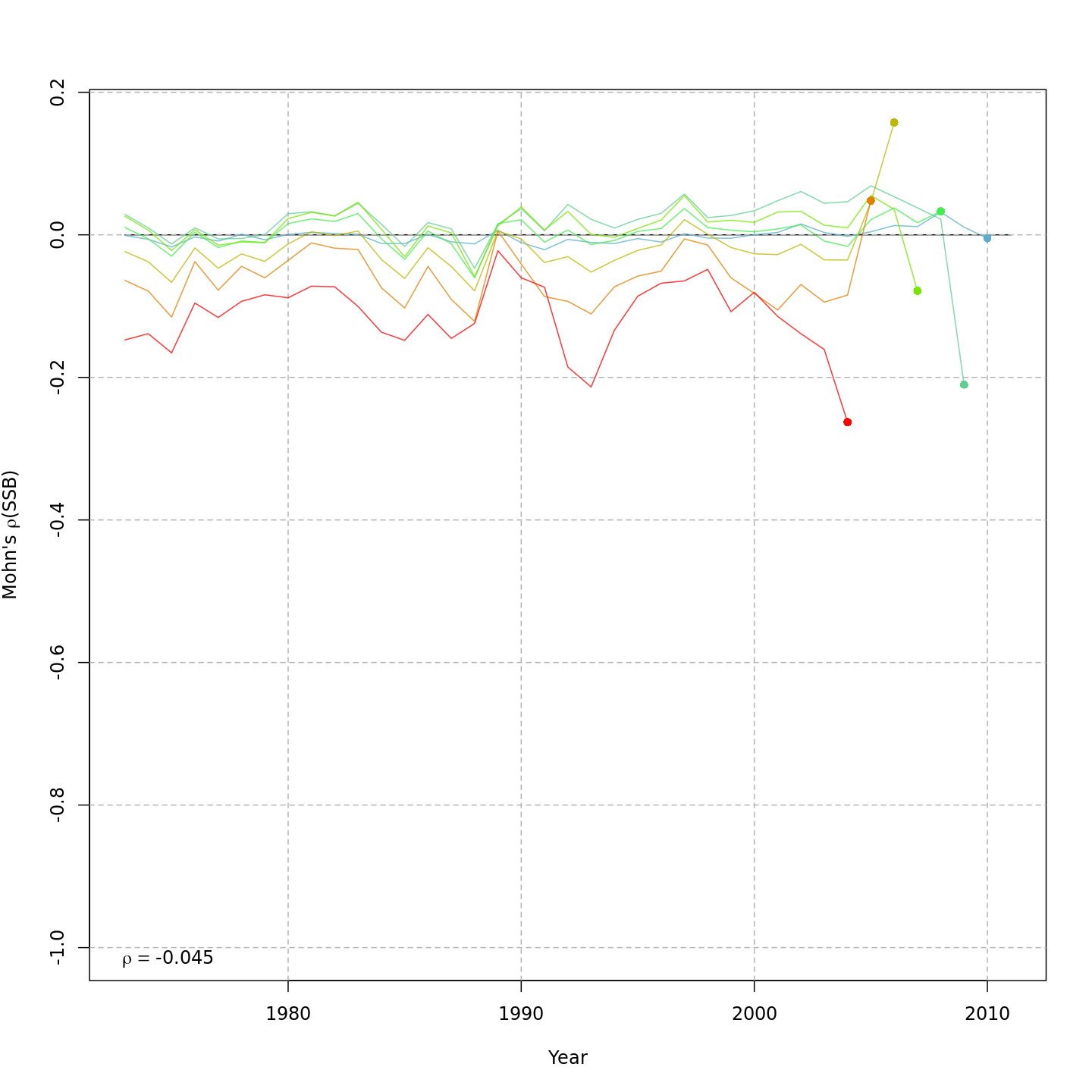
Retrospective patterns

Compared to m1, the retrospective pattern for m8 was slightly worse for recruitment (m8 0.32, m1 0.23) but improved for SSB (m8 0.01, m1 0.07) and F (m8 -0.05, m1 -0.11). In general, models with GSI effects or 2D AR1 deviations on $M$ had reduced retrospective patterns compared to the status quo (m1) and models with 1D AR1 random effects on $M$. Compare the retrospective patterns of numbers-at-age, SSB, and F for models m1 (left, fixed $M_a$) and m8 (right, estimated $M$ + 2D AR1 deviations).

Mohn’s rho for numbers-at-age, m1.

Mohn’s rho for SSB, m1. Mohn’s rho for SSB, m8.

Mohn’s rho for F, m1. Mohn’s rho for F, m8.

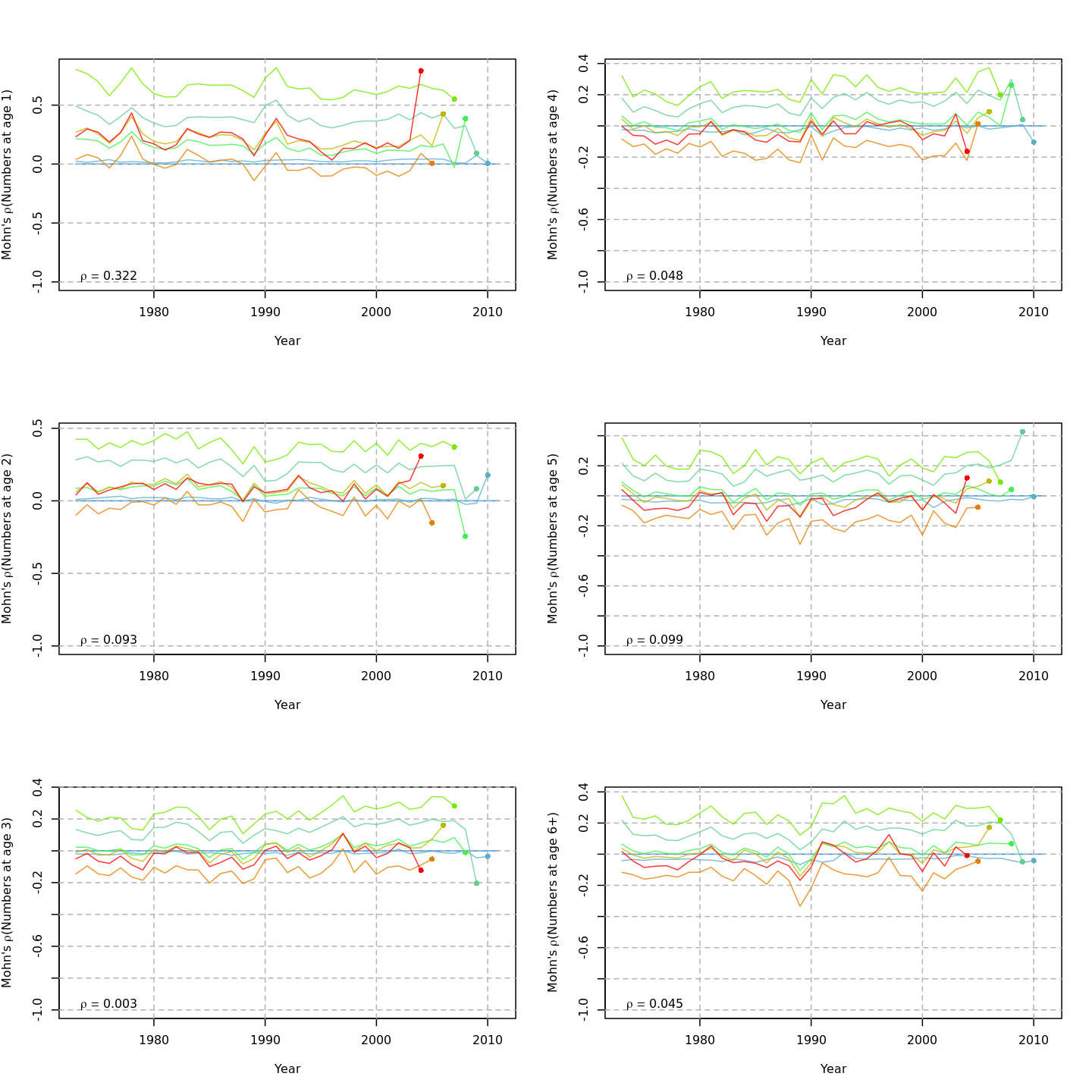
Model m11 had $\Delta AIC = 1.5$ and the lowest retrospective pattern for all numbers-at-age and F. Model m11 left $M_a$ fixed at the values from the ASAP data file (as in m1) and estimated 2D AR1 deviations around these mean $M_a$. This is how $M$ was modeled in Cadigan (2016).

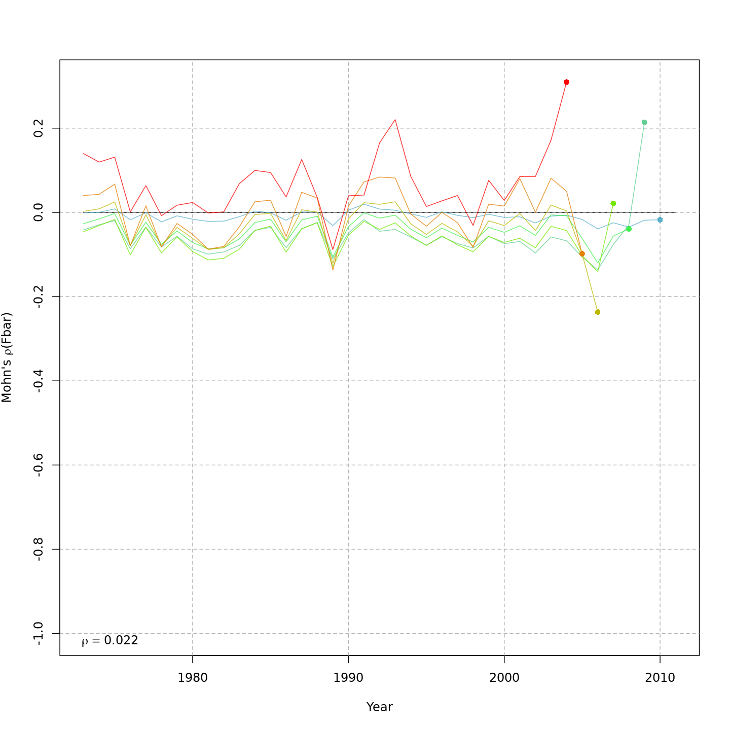
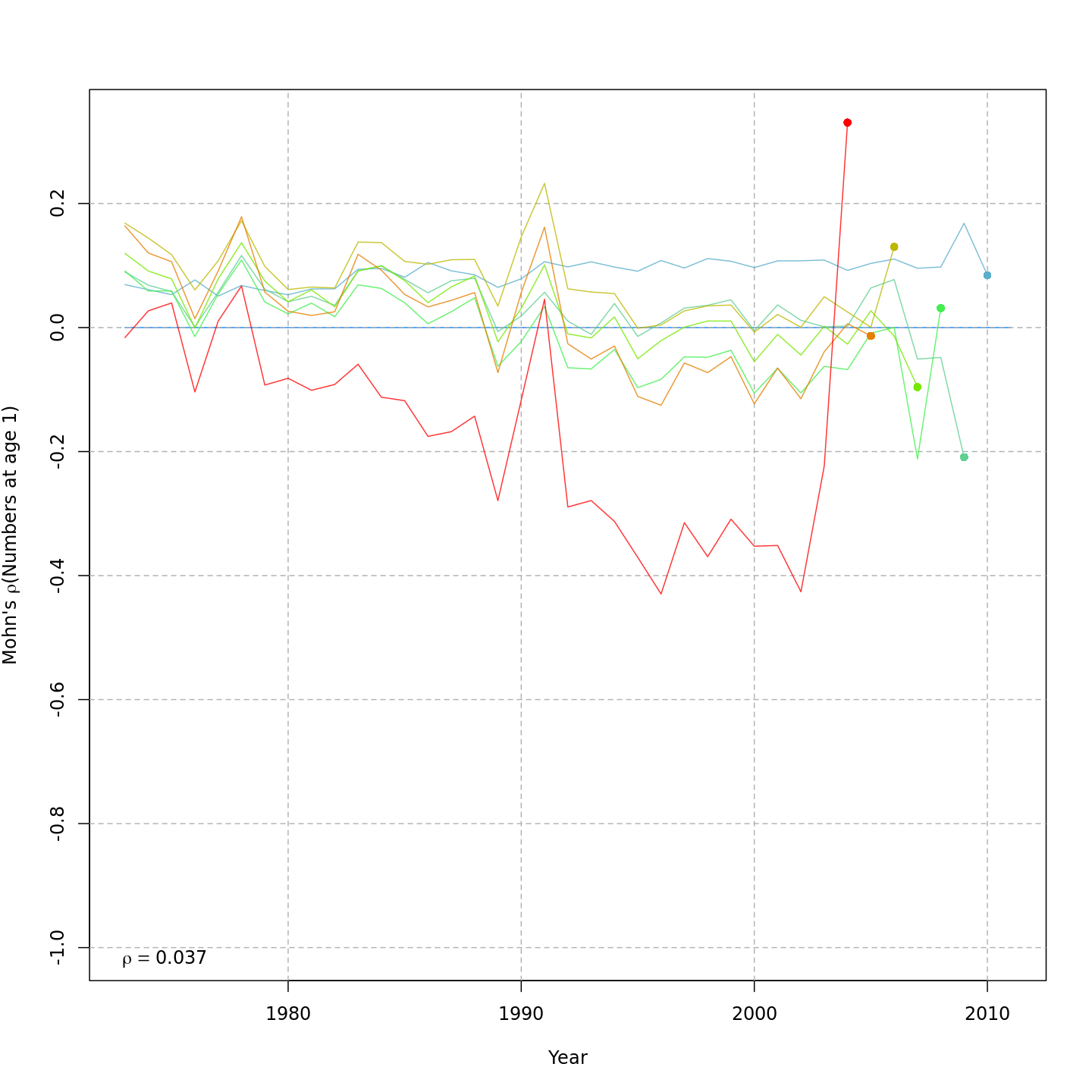
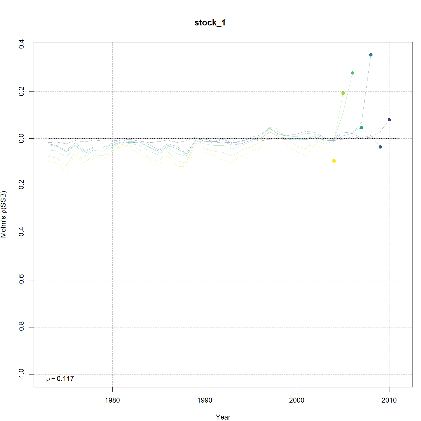
Mohn’s rho for SSB, m11. Mohn’s rho for F, m11.

Mohn’s rho for recruitment, m11.

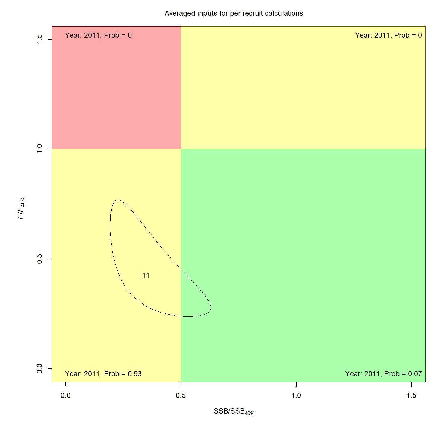
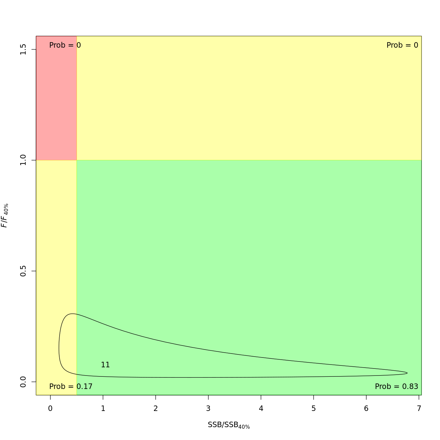
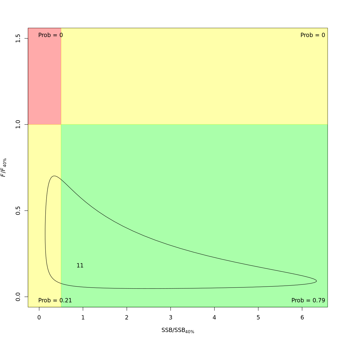
Stock status

Compared to m1 (left), m8 and m11 (center, right) estimated higher M, lower and more uncertain F, and higher SSB – a much rosier picture of the stock status through time.

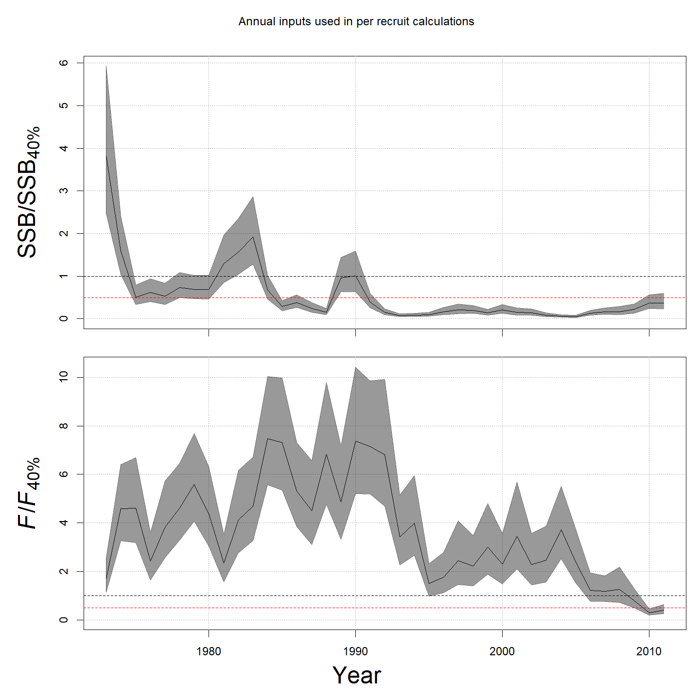
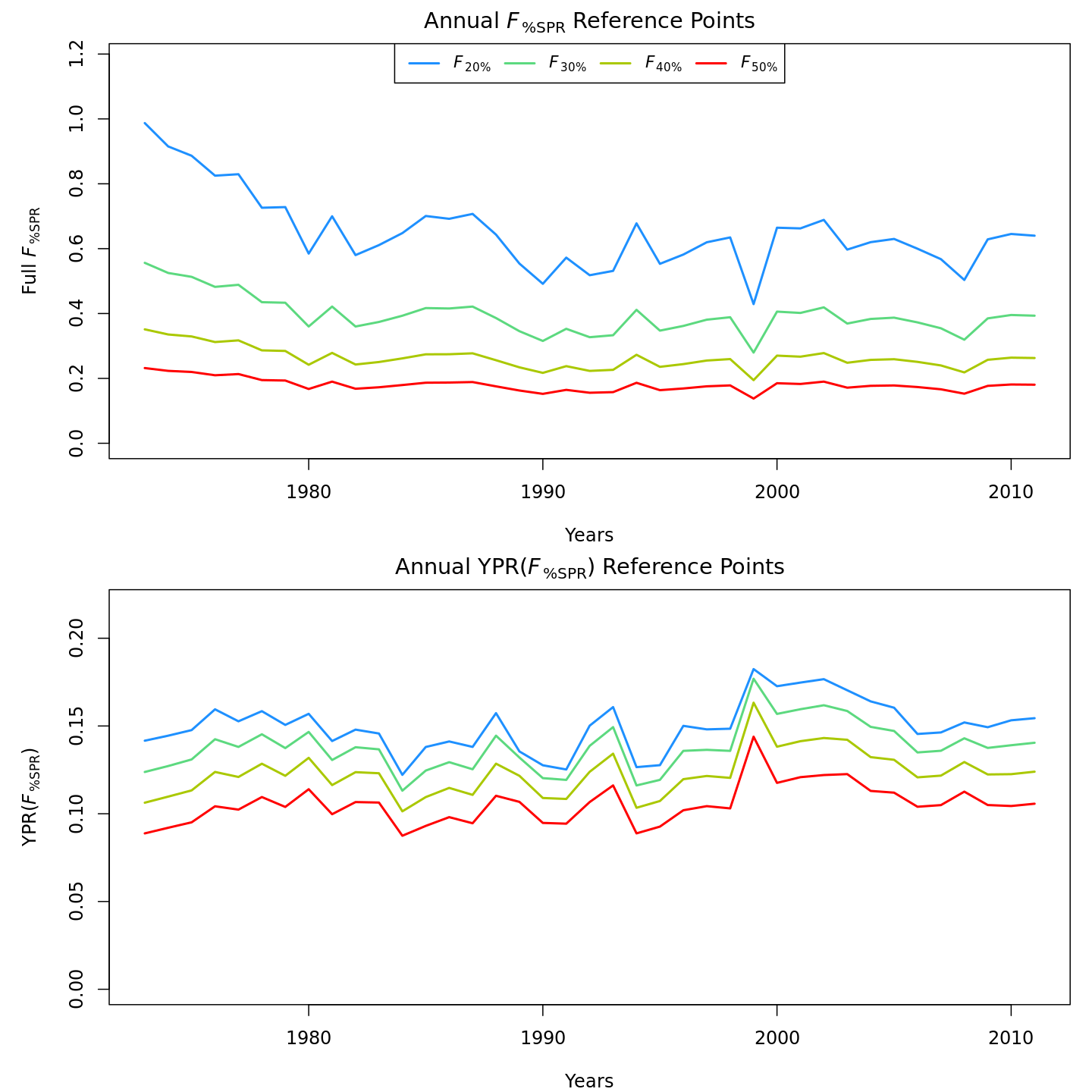
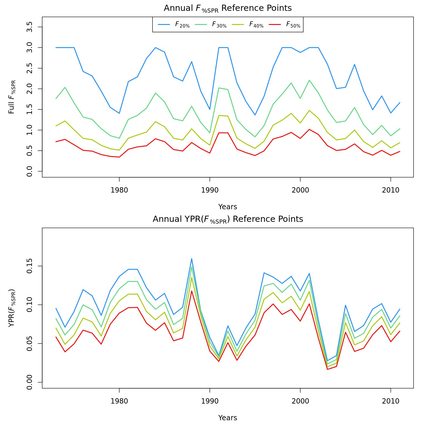
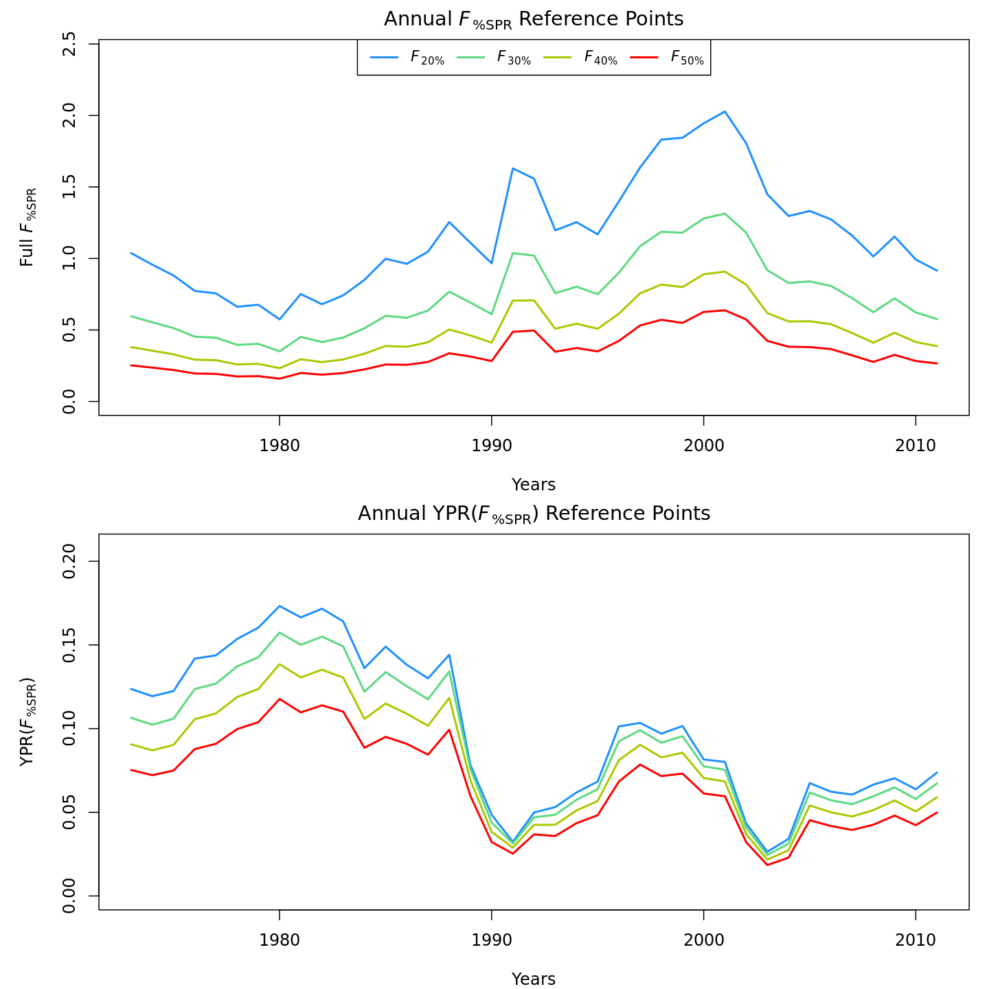
Relative stock status, m1. Relative stock status, m8. Relative stock status, m11.

Compared to m1 (left), m8 and m11 (center, right) estimated higher and more variable reference points, $F_{\%SPR}$ (top), and lower and more variable yield-per-recruit (bottom). Model m11 (right) estimated more of a trend in yield-per-recruit and $F_{\%SPR}$, with a notable shift around 1990.

Reference point variability, m1.

In the final year (2011), m8 and m11 both estimated much lower probabilities of the stock being overfished than m1 (17% and 21% vs. 99%).

Kobe status plot, m1. Kobe status plot, m8. Kobe status plot, m11.

Yet more M options

If you want to estimate M-at-age shared/mirrored among some but not all ages, you’ll need to modify input$map$M_a after calling prepare_wham_input().