Ex 1: The basics

In this vignette we walk through an example using the wham (WHAM = the Woods Hole Assessment Model) package to run a state-space age-structured stock assessment model. WHAM is a generalization of code written for Miller et al. (2016), and in this example we apply WHAM to the same stock as in Miller et al. (2016), Southern New England / Mid-Atlantic Yellowtail Flounder. Here, we demonstrate the basic wham workflow:

Load wham and data
Specify several (slightly different) models:
- m1: statistical catch-at-age (SCAA) model, but with recruitment estimated as random effects; multinomial age-compositions
- m2: as m1, but with logistic normal age-compositions
- m3: full state-space model (numbers at all ages are random effects), multinomial age-compositions
- m4: full state-space model, logistic normal age-compositions
Fit models and check for convergence
Compare models by AIC and Mohn’s rho (retrospective analysis)
Review plots of input data, diagnostics, and results.

1. Load data

We assume you have already read the Introduction and installed wham and its dependencies. If not, you should be able to install using the remotes or pak packages: remotes::install_github("timjmiller/wham", dependencies=TRUE). pak::pkg_install("timjmiller/wham")

Open R and load the wham package:

library(wham)

For a clean, runnable .R script, look at ex1_basics.R in the example_scripts folder of the wham package. You can run this entire example script with:

wham.dir <- find.package("wham")
source(file.path(wham.dir, "example_scripts", "ex1_basics.R"))

Let’s create a directory for this analysis:

# choose a location to save output, otherwise will be saved in working directory
write.dir <- "choose/where/to/save/output" #e.g., tempdir(check=TRUE)
dir.create(write.dir)
setwd(write.dir)

WHAM was built by modifying the ADMB-based ASAP model code (Legault and Restrepo 1999), and is designed to take an ASAP3 .dat file as input. We generally assume in wham that you have an existing ASAP3 .dat file. If you are not familiar with ASAP3 input files, see the ASAP documentation and code. For this vignette, an example ASAP3 input file is provided.

Read the ASAP3 .dat file into R:

path_to_examples <- system.file("extdata", package="wham")
asap3 <- read_asap3_dat(file.path(path_to_examples,"ex1_SNEMAYT.dat"))

2. Specify model

We use the prepare_wham_input() function to specify the model name and any settings that differ from the ASAP3 file. Our first model will use:

recruitment model: random about mean, no S-R function (recruit_model = 2)
recruitment deviations: independent random effects (NAA_re = list(sigma="rec", cor="iid"))
selectivity: age-specific (fix sel=1 for ages 4-5 in fishery, age 4 in index1, and ages 2-4 in index2)

input1 <- prepare_wham_input(asap3, recruit_model=2, model_name="Ex 1: SNEMA Yellowtail Flounder",
  selectivity=list(model=rep("age-specific",3), 
    re=rep("none",3), 
    initial_pars=list(c(0.5,0.5,0.5,1,1,0.5),c(0.5,0.5,0.5,1,0.5,0.5),c(0.5,1,1,1,0.5,0.5)), 
    fix_pars=list(4:5,4,2:4)),
  NAA_re = list(sigma="rec", cor="iid"))

Note the text that is printed to the console by this command. The function attempts to provide some description of assumptions being made for this model configuration as well as some changes in default configurations in recent versions.

The stock-recruit model options in WHAM are:

1 = random walk,
2 = random about mean (default),
3 = Beverton-Holt, and
4 = Ricker

Note that the parameterization of age-specific selectivity is specific to SNEMA yellowtail flounder. We will use age-specific selectivity parameters for the first three selectivity blocks. Selectivity blocks define a selectivity configuration that can be used in one or more fleets or surveys over any set of years in the model. prepare_wham_input() fixes age-specific parameters at zero if there are any age classes without any observations where the selectivity block is applied. The function configures all other age-specific parameters to be estimated. Generally there may be confounding of the selectivity parameters with either fully-selected fishing mortality (for fleets) or catchability (for surveys), so selectivity parameters for one or more ages would need to be fixed to allow convergence. An initial fit with all selectivity parameters freely estimated can be useful in determining which age(s) to fix selectivity at 1. In the code above, we have already determined the ages to fix selectivity at 1 (ages 4-5 in fishery, age 4 in index 1, and ages 2-4 in index 2). If you are interested in more details and options for selectivity in WHAM, see Example 4 and prepare_wham_input().

3. Fit model and check for convergence

m1 <- fit_wham(input1, do.osa = F) # turn off OSA residuals to save time in ex

By default, fit_wham() uses 3 extra Newton steps to reduce the absolute value of the gradient (n.newton = 3) and estimates standard errors for derived parameters (do.sdrep = TRUE). fit_wham() also does a retrospective analysis with 7 peels by default (do.retro = TRUE, n.peels = 7). For more details, see fit_wham().

We need to check that m1 converged (m1$opt$convergence should be 0, and the maximum absolute value of the gradient vector should be < 1e-06). Convergence issues may indicate that a model is misspecified or overparameterized. To help diagnose these problems, fit_wham() includes a do.check option to run an internal check_estimability function originally written by Jim Thorson. do.check = FALSE by default. To turn on, set do.check = TRUE. See fit_wham().

check_convergence(m1)

#> stats:nlminb thinks the model has converged: mod$opt$convergence == 0
#> Maximum gradient component: 1.56e-12 
#> Max gradient parameter: logit_q 
#> TMB:sdreport() was performed successfully for this model

Fit models `m2`-`m4`

The second model, m2, is like the first, but changes all the age composition likelihoods from multinomial to logistic normal (treating 0 observations as missing):

input2 <- prepare_wham_input(asap3, recruit_model=2, model_name="Ex 1: SNEMA Yellowtail Flounder",
  selectivity=list(model=rep("age-specific",3), 
    re=rep("none",3), 
    initial_pars=list(c(0.5,0.5,0.5,1,1,0.5),c(0.5,0.5,0.5,1,0.5,0.5),c(0.5,1,1,1,0.5,0.5)), 
    fix_pars=list(4:5,4,2:4)),
  NAA_re = list(sigma="rec", cor="iid"),
  age_comp = "logistic-normal-miss0")
m2 <- fit_wham(input2, do.osa = F) # turn off OSA residuals to save time

Check that m2 converged:

check_convergence(m2)

#> stats:nlminb thinks the model has converged: mod$opt$convergence == 0
#> Maximum gradient component: 1.03e-11 
#> Max gradient parameter: index_paa_pars 
#> TMB:sdreport() was performed successfully for this model

The third, m3, is a full state-space model where numbers at all ages are random effects (NAA_re$sigma = "rec+1"):

input3 <- prepare_wham_input(asap3, recruit_model=2, model_name="Ex 1: SNEMA Yellowtail Flounder",
  selectivity=list(model=rep("age-specific",3), 
    re=rep("none",3), 
    initial_pars=list(c(0.5,0.5,0.5,1,1,0.5),c(0.5,0.5,0.5,1,0.5,0.5),c(0.5,1,1,1,0.5,0.5)), 
    fix_pars=list(4:5,4,2:4)),
  NAA_re = list(sigma="rec+1", cor="iid"))
m3 <- fit_wham(input3, do.osa = F) # turn off OSA residuals to save time

Check that m3 converged:

check_convergence(m3)

#> stats:nlminb thinks the model has converged: mod$opt$convergence == 0
#> Maximum gradient component: 3.04e-11 
#> Max gradient parameter: logit_selpars 
#> TMB:sdreport() was performed successfully for this model

The last, m4, is like m3, but again changes all the age composition likelihoods to logistic normal:

input4 <- prepare_wham_input(asap3, recruit_model=2, model_name="Ex 1: SNEMA Yellowtail Flounder",
  selectivity=list(model=rep("age-specific",3), 
    re=rep("none",3), 
    initial_pars=list(c(0.5,0.5,0.5,1,1,0.5),c(0.5,0.5,0.5,1,0.5,0.5),c(0.5,1,1,1,0.5,0.5)), 
    fix_pars=list(4:5,4,2:4)),
  NAA_re = list(sigma="rec+1", cor="iid"),
  age_comp = "logistic-normal-miss0")
m4 <- fit_wham(input4, do.osa = F) # turn off OSA residuals to save time

Check that m4 converged: The max absolute gradient is not good.

check_convergence(m4)

#> stats:nlminb thinks the model has NOT converged: mod$opt$convergence != 0
#> Maximum gradient component: 9.97e-01 
#> Max gradient parameter: F_pars 
#> TMB:sdreport() was not performed for this model

Try refitting starting at the previously estimated values. This helps sometimes.

input4$par <- m4$parList #best estimates so far
m4_good <- fit_wham(input4, do.osa = F) # turn off OSA residuals to save time

Now convergence is good.

check_convergence(m4_good)

#> stats:nlminb thinks the model has converged: mod$opt$convergence == 0
#> Maximum gradient component: 2.40e-10 
#> Max gradient parameter: index_paa_pars 
#> TMB:sdreport() was performed successfully for this model

Now, add the One-step-ahead residuals to the model fit using the make_osa_residuals function

m4_good <- make_osa_residuals(m4_good) #returns the model with the residuals added.

Store all models together in one (named) list:

mods <- list(m1=m1, m2=m2, m3=m3, m4=m4_good)

Since the retrospective analyses take a few minutes to run, you may want to save the output for later use:

save("mods", file="ex1_models.RData")

4. Compare models

compare_wham_models() will make 1) a table comparing multiple WHAM model fits using AIC and Mohn’s rho, and 2) plots of key output (e.g. SSB, F, recruitment, reference points).

res <- compare_wham_models(mods, table.opts=list(fname="ex1_table", sort=TRUE))

#>      dAIC     AIC  rho_R rho_SSB rho_Fbar
#> m4    0.0 -1472.4 0.3474  0.0584  -0.0416
#> m2  306.0 -1166.4 5.1190 -0.0205   0.0174
#> m3 5573.6  4101.2 0.1271  0.0290  -0.0230
#> m1 6312.9  4840.5 0.8207  0.1840  -0.1748

res$best

#> [1] "m4"

By default, compare_wham_models() sorts the model comparison table with lowest (best) AIC at the top, and saves it as model_comparison.csv. However, in this example the models with alternative likelihoods for the age composition observations are not comparable due to differences in how the observations are defined. Still, the models that treat the age composition observations in the same way can be compared to evaluate whether stochasticity in abundances at age provides better performance, i.e. m1 vs. m3 (both multinomial) and m2 vs. m4 (both logistic normal).

The comparison plots are stored by default in the compare_png folder.

Project the best model

Let’s do projections for the best model, m4, using the default settings (see project_wham()):

m4_proj <- project_wham(model=m4)

5. Plot input data, diagnostics, and results

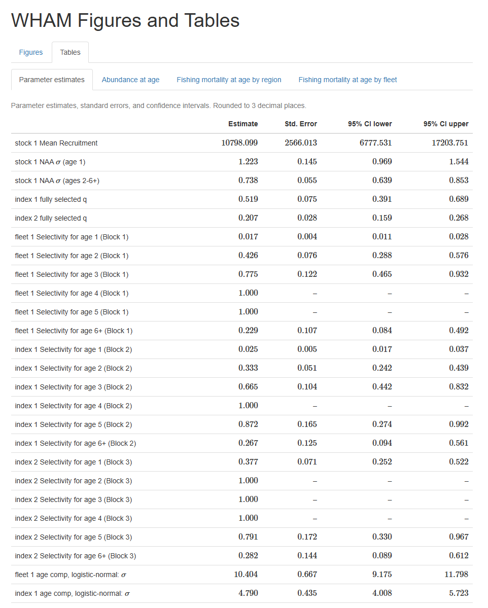
There are various options for creating WHAM output. The default is to create a self-contained html file using Rmarkdown and individual plot files (.png) that are organised within subdirectories of plots_png. The html file also includes tables of estimates for fundamental parameters and abundance and fishing mortality at age. On Windows you may need to use Chrome or Internet Explorer to view the .html (there have been issues using Firefox on Windows but not Linux).

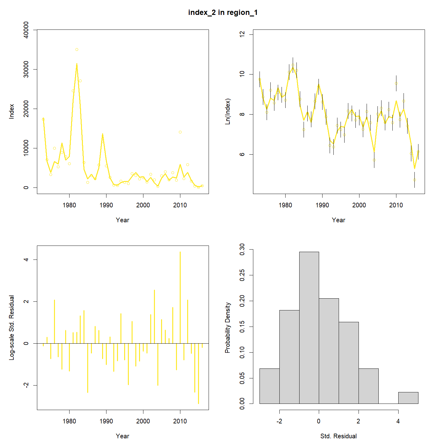
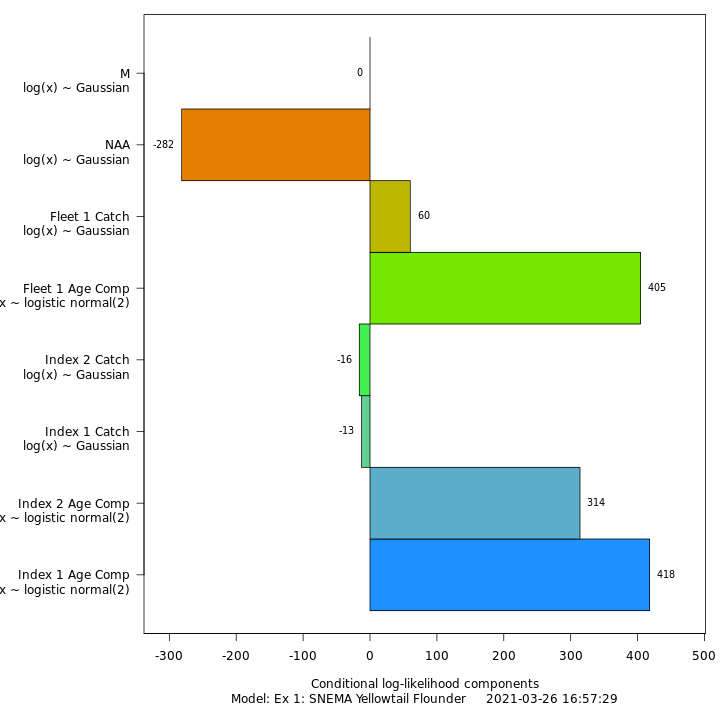
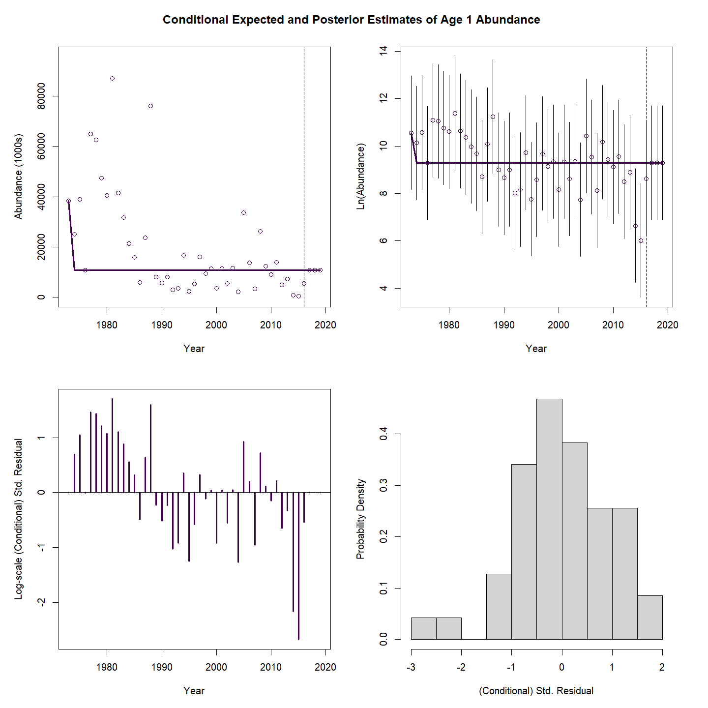
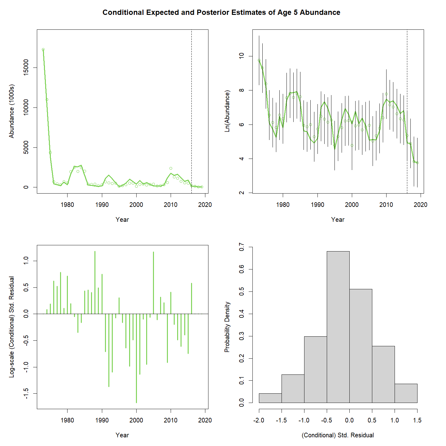
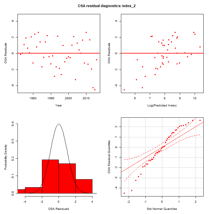
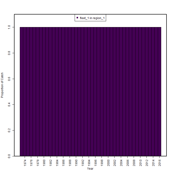
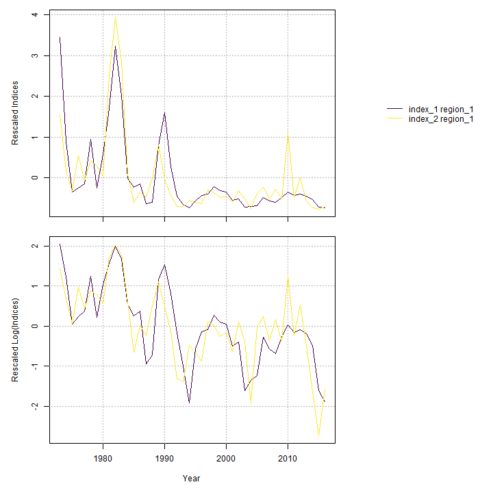
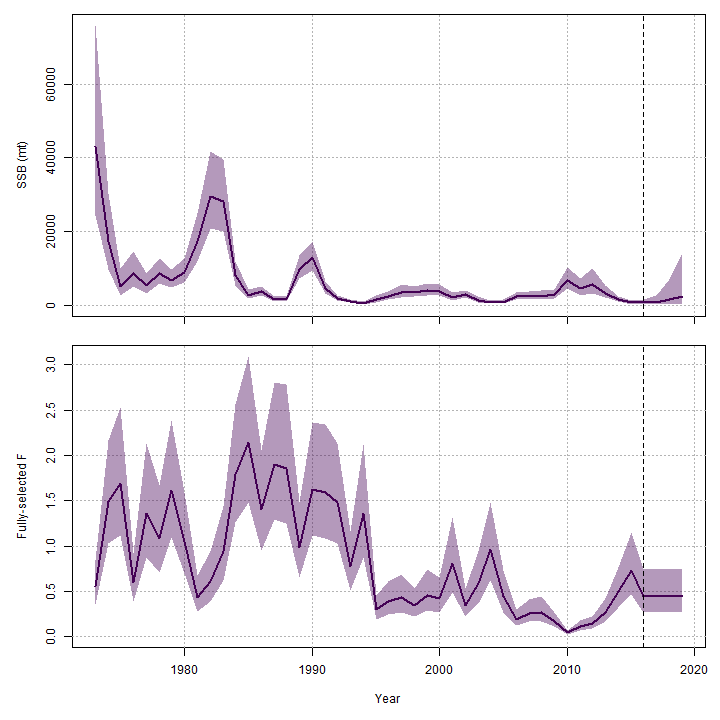
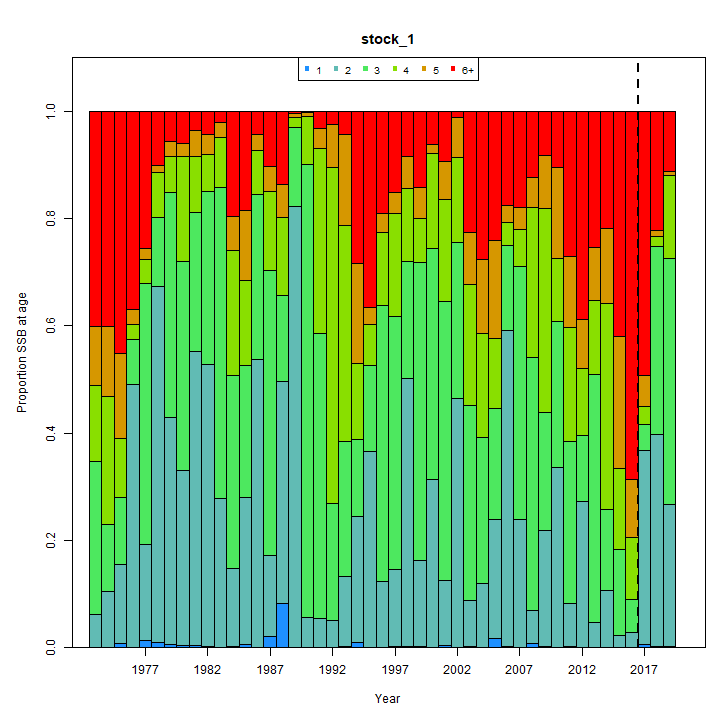
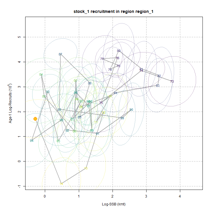
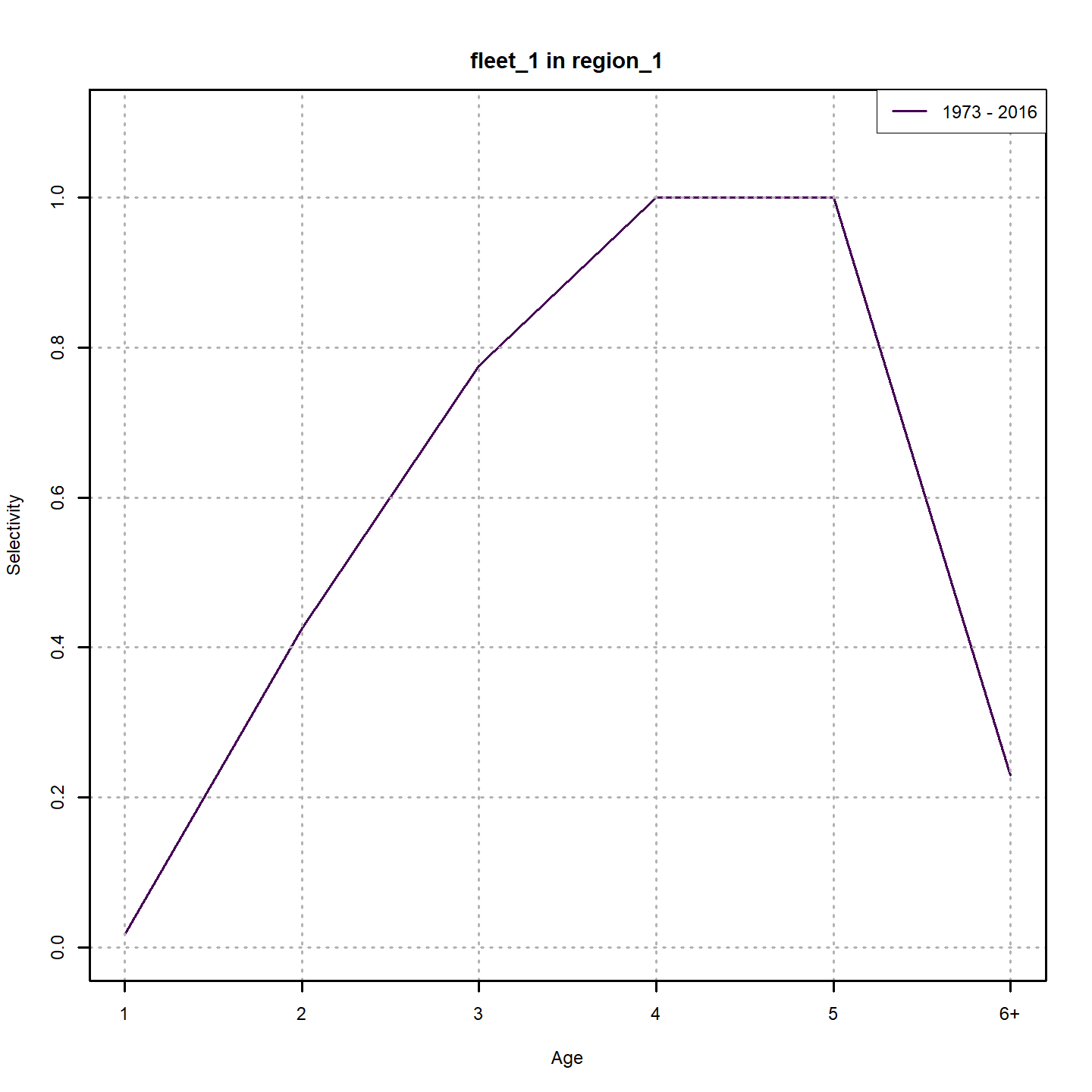
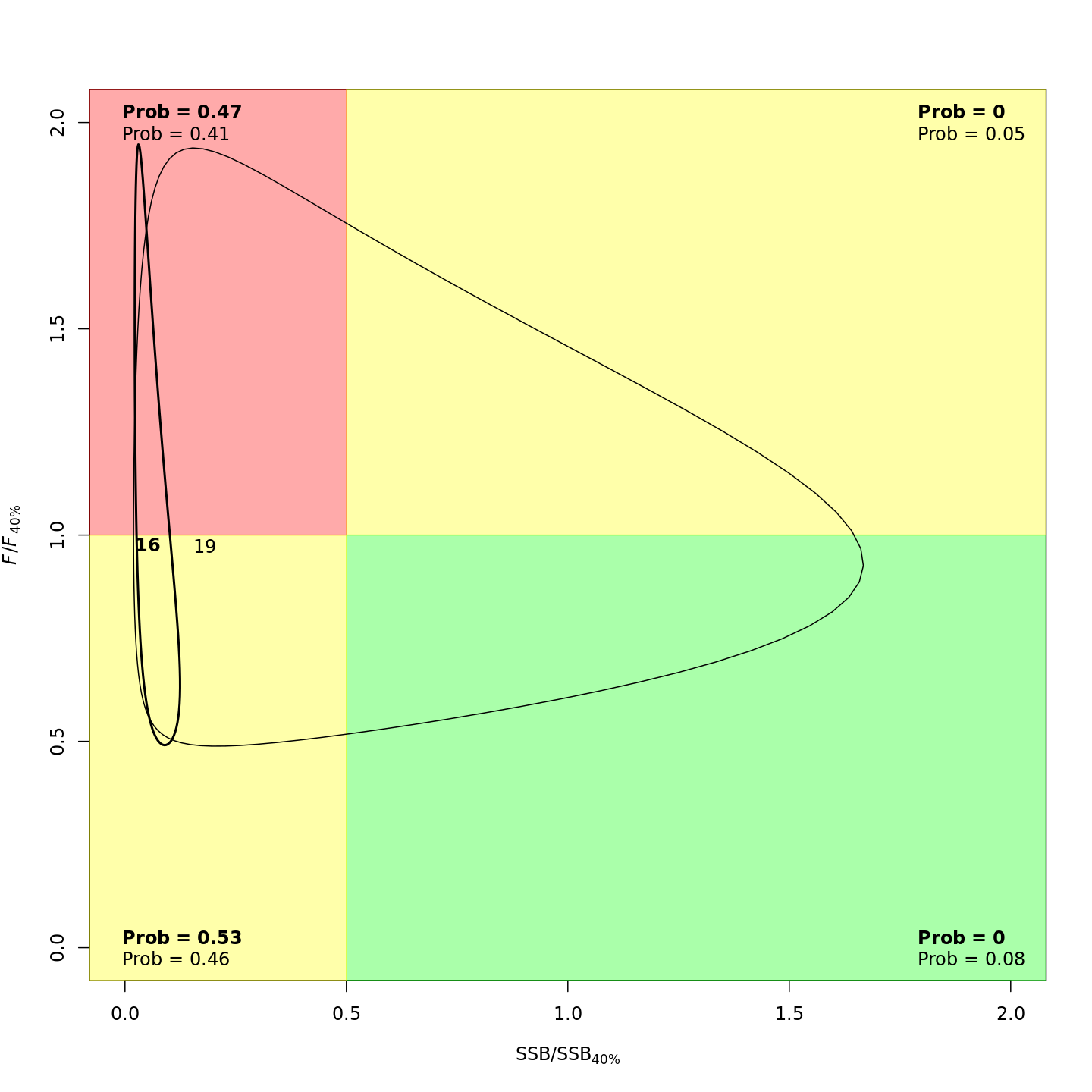
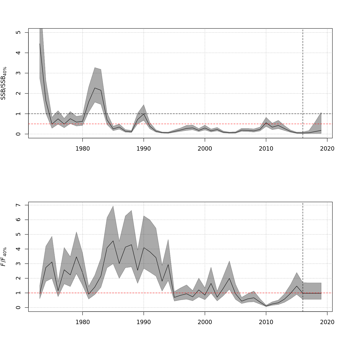
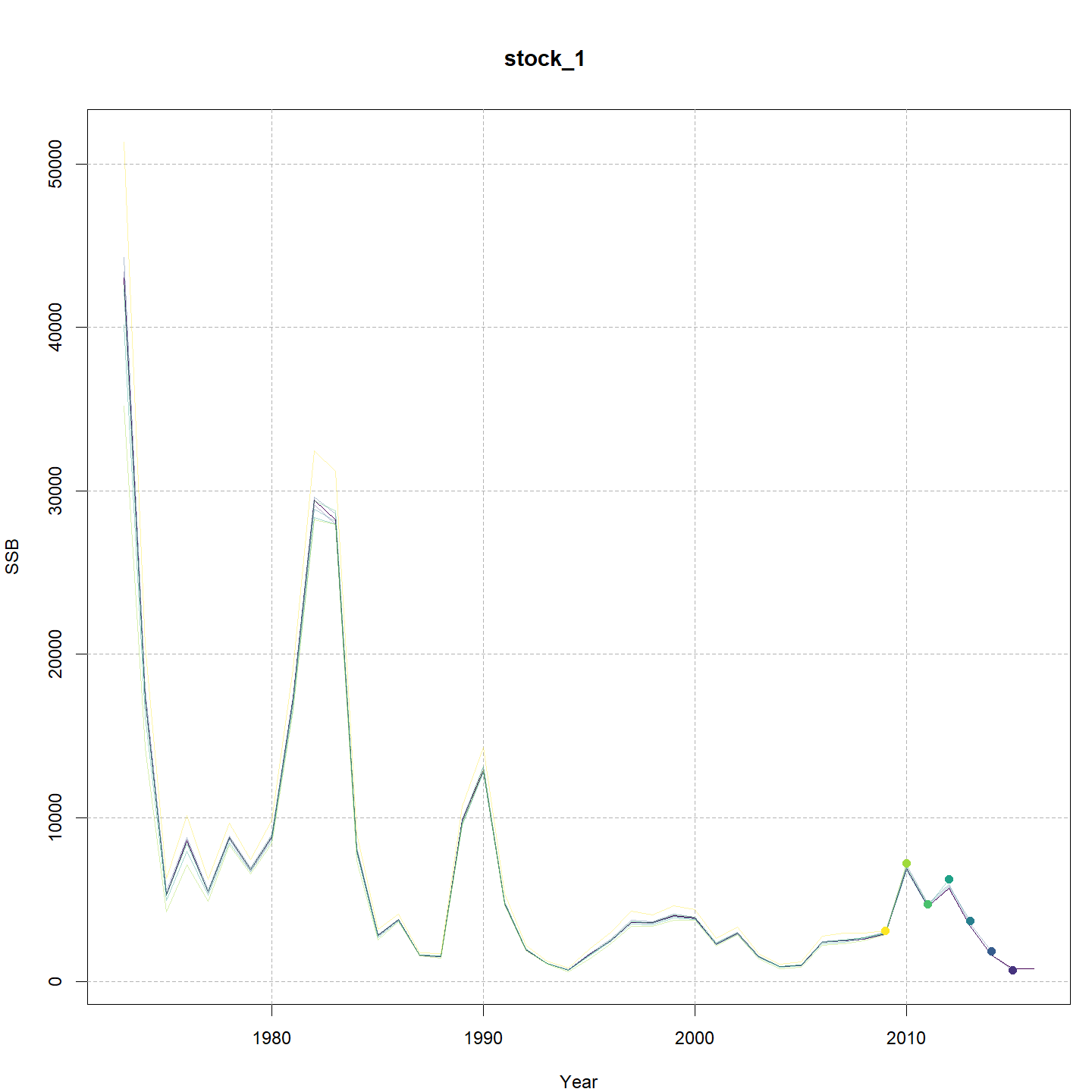
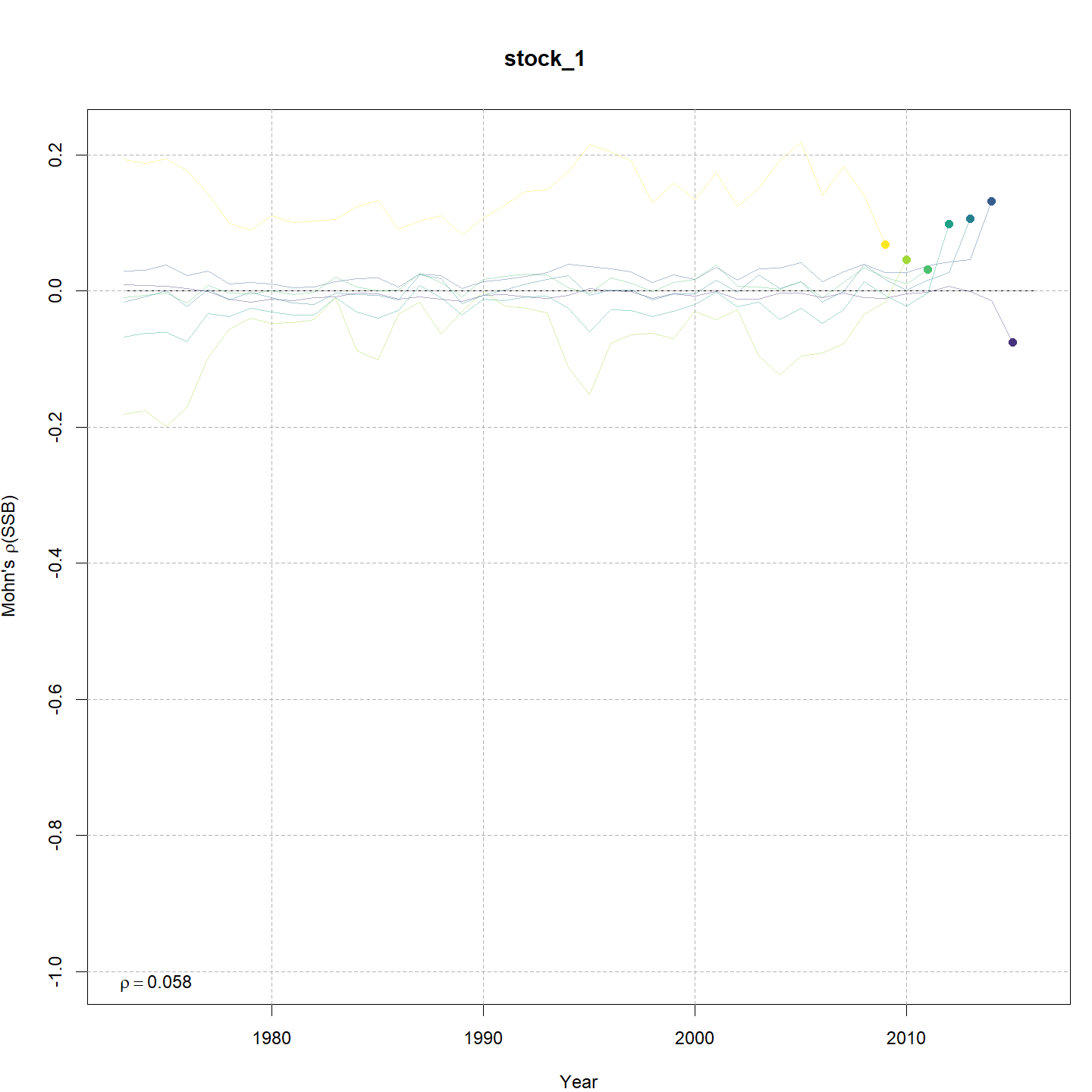
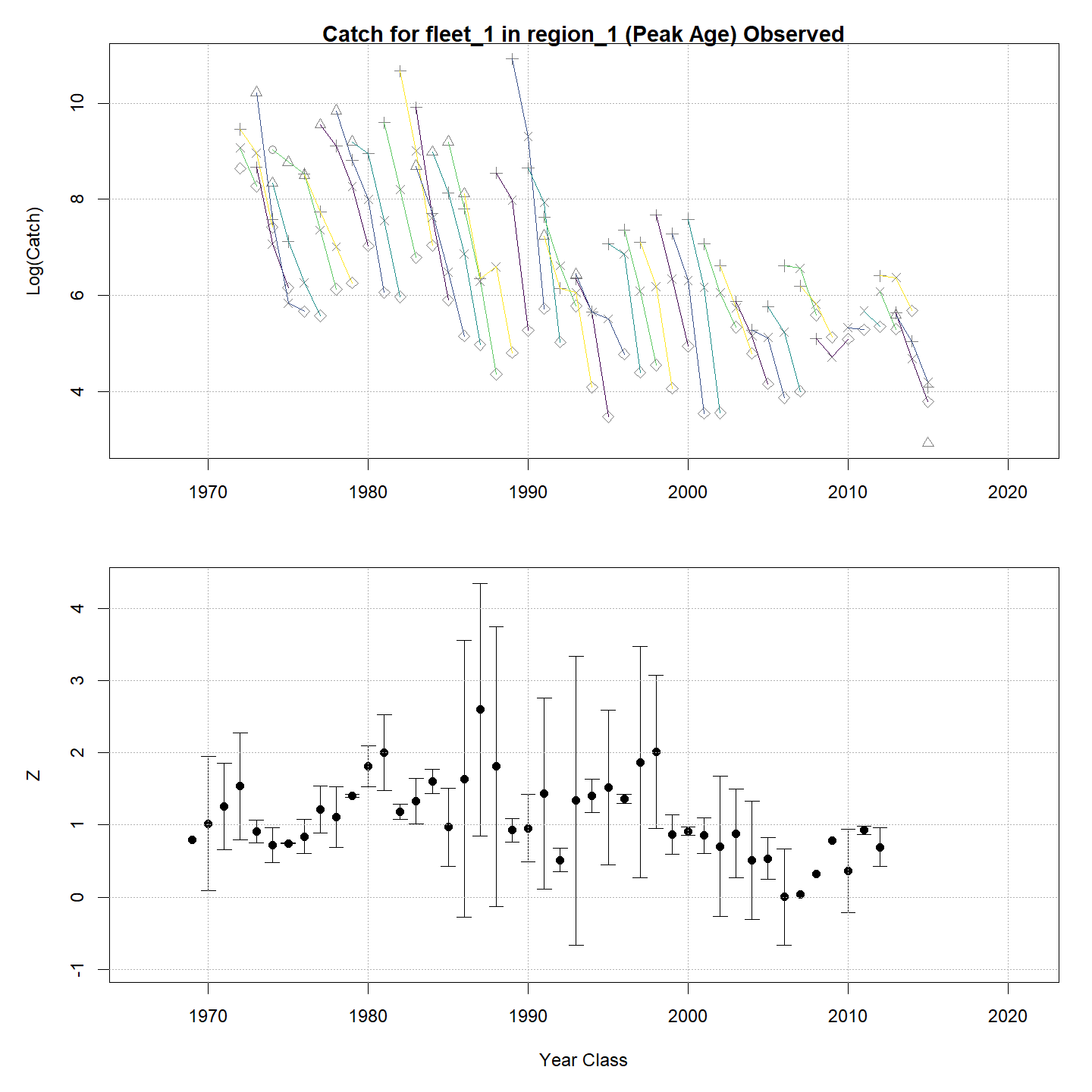
plot_wham_output(mod=m4_proj, out.type='html') #default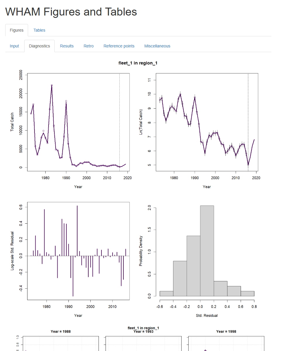

Example HTML file created by plot_wham_output(mod=m4, out.type='html') for plots.

Example HTML file created by plot_wham_output(mod=m4, out.type='html') for tables.

Setting out.type='pdf' saves the plots organized into 6 .pdf files corresponding to the tabs in the .html file (Diagnostics, Input Data, Results, Reference Points, Retrospective, and Misc). This option will also generate a pdf of the same tables as those under the html option.

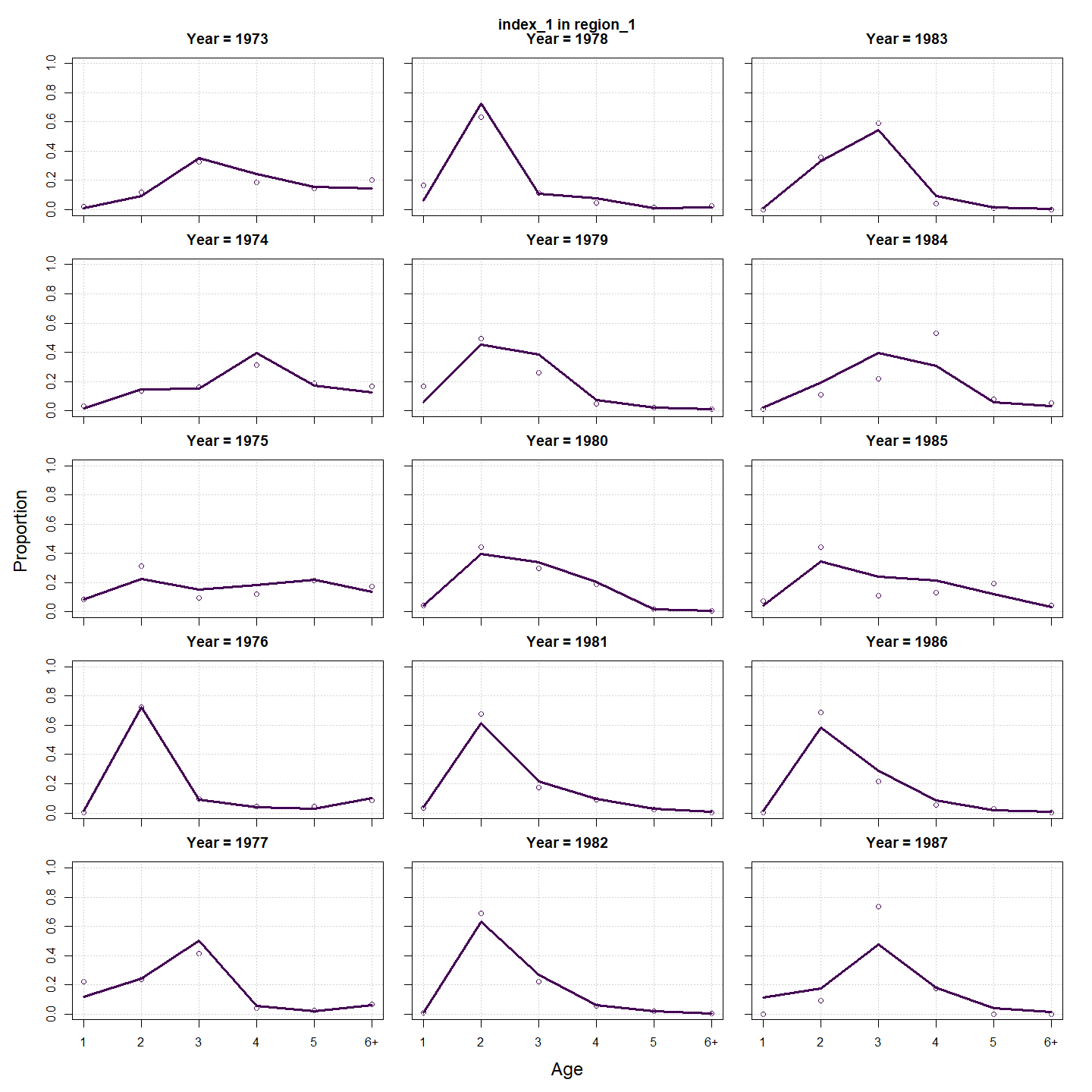
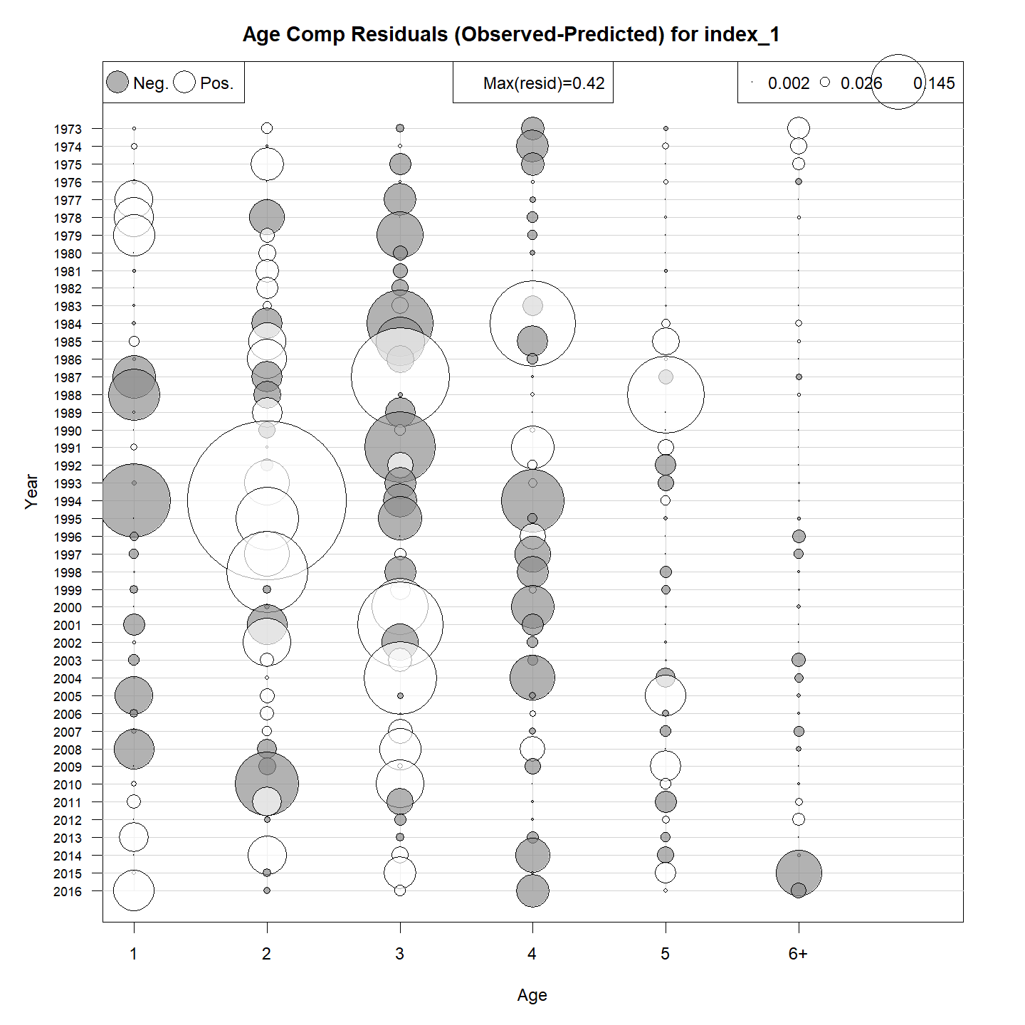
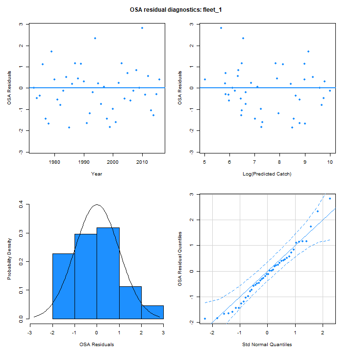
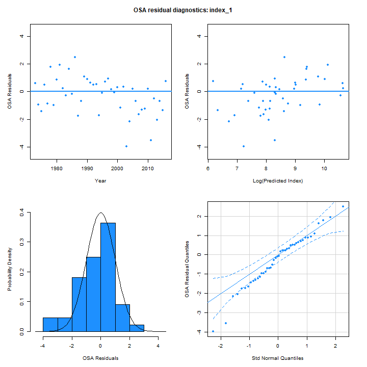
Many plots are generated—here we display some examples: