1. Background
In this vignette we show how to use WHAM for general simulation
studies. It updateds and replaces a previous WHAM vignette on Operating
models and MSE. We assume you already have wham installed
and are relatively familiar with the package. If not, read the Introduction and Tutorial.
In this vignette we show how to:
- Simulate data from a fitted model with input derived from an ASAP3 dat file.
- Make an operating model, simulate data, and fit models.
- Fit models to data simulated from a different model.
- Make a wham input file without an ASAP3 dat file.
- Configure different assumptions about the population for both the operating model and the estimating model.
- Do a closed-loop simulation with operating model, fitting an estimating model, generating catch advice and incorporating it into the operating model.
2. Setup and read in model input
Create a directory for this analysis:
# choose a location to save output, otherwise will be saved in working directory
write.dir <- "choose/where/to/save/output"
dir.create(write.dir)
setwd(write.dir)
wham.dir <- find.package("wham")
asap3 <- read_asap3_dat(file.path(wham.dir,"extdata","ex1_SNEMAYT.dat"))
Make an input and fit a model in wham. This model was also fit in the first example vignette.
#define selectivity model
selectivity=list(
  model=rep("age-specific",3), #define selectivity model
  re=rep("none",3), #define selectivity random effects model
  #define initial/fixed values for age-specific selectivity
  initial_pars=list(c(0.5,0.5,0.5,1,1,0.5),c(0.5,0.5,0.5,1,0.5,0.5),c(0.5,1,1,1,0.5,0.5)),
  fix_pars=list(4:5,4,2:4)) #which ages to not estimate age-specfic selectivity parameters

NAA_re = list(
  sigma="rec", #random effects for recruitment only
  cor="iid", #random effects are independent
  recruit_model = 2) #mean recruitment is the only fixed effect parameter

input <- prepare_wham_input(
  asap3,
  selectivity = selectivity,
  NAA_re = NAA_re,
  model_name="Ex 1: SNEMA Yellowtail Flounder")

mod_1 <- fit_wham(input, do.osa = FALSE, do.retro=FALSE, MakeADFun.silent = TRUE) # don't do retro peels and OSA residuals, don't show output during optimization
names(mod_1)
#>  [1] "par"            "fn"             "gr"             "he"
#>  [5] "hessian"        "method"         "retape"         "env"
#>  [9] "report"         "simulate"       "years"          "years_full"
#> [13] "ages.lab"       "model_name"     "input"          "call"
#> [17] "rep"            "wham_commit"    "wham_version"   "opt"
#> [21] "date"           "dir"            "TMB_commit"     "TMB_version"
#> [25] "parList"        "final_gradient" "is_sdrep"       "na_sdrep"
#> [29] "runtime"        "sdrep"
Several of the elements in the object returned by
fit_wham are those produced by TMB::MakeADFun.
mod_1$par are the fixed effects or parameters over which
the marginal likelihood is optimized. mod_1$fn is the
function that returns the (Laplace approximation of) the negative
marginal log-likelihood. mod_1$gr is the function that
returns the gradient and mod_1$he returns the hessian.
mod_1$report is a function that provides a list of output
defined by REPORT() calls in the compiled cpp code and is already
evaluated and provided by mod_1$rep. When available,
mod_1$sdrep provides the hessian based standard errors for
estimates from the model which is generated by
theTMB::sdreport function.
mod_1$sdrep #the standard errors of the fixed effects
#>                    Estimate Std. Error
#> mean_rec_pars  9.2297317468 0.20741202
#> logit_q       -7.6658675842 0.07240548
#> logit_q       -8.3316202926 0.04787635
#> F_pars        -0.3010365597 0.10378094
#> F_pars         0.9285229416 0.13406941
#> F_pars        -0.0004773479 0.12741677
#> F_pars        -0.6333646293 0.14063536
#> F_pars         0.3545992256 0.15672409
#> F_pars         0.0007498385 0.14814836
#> F_pars        -0.1186869337 0.13952459
#> F_pars        -0.3135424185 0.13573691
#> F_pars        -0.3638492439 0.14032728
#> F_pars         0.3747984450 0.15107794
#> F_pars         0.4062432156 0.14131528
#> F_pars         0.3345658415 0.12315402
#> F_pars        -0.0926085078 0.12354231
#> F_pars        -0.0268561987 0.12975421
#> F_pars        -0.1547492535 0.13236249
#> F_pars        -0.5781912378 0.14060717
#> F_pars         0.0729322405 0.14723880
#> F_pars         0.5728244469 0.13078407
#> F_pars        -0.1306285071 0.11004614
#> F_pars        -0.2800617478 0.11369600
#> F_pars        -0.5485798871 0.12377094
#> F_pars         0.3737751961 0.13772134
#> F_pars        -0.9198984028 0.13376737
#> F_pars         0.2580256177 0.14685907
#> F_pars         0.4837561008 0.14669630
#> F_pars        -0.0965007661 0.14584155
#> F_pars         0.1868119330 0.15441950
#> F_pars        -0.0813445695 0.15144239
#> F_pars         0.1925950197 0.15297110
#> F_pars        -0.4368514619 0.14045843
#> F_pars        -0.1981206595 0.14133134
#> F_pars         0.2086433955 0.14571752
#> F_pars        -0.5430209898 0.13831609
#> F_pars        -0.2223686593 0.14787653
#> F_pars        -0.3312150849 0.14530564
#> F_pars        -0.1132458326 0.14270517
#> F_pars        -0.3259619687 0.13965183
#> F_pars        -0.3070878804 0.14247434
#> F_pars         0.4437180306 0.14646439
#> F_pars         0.4592751847 0.14826234
#> F_pars         0.3692754247 0.15160407
#> F_pars         0.2753424755 0.15409611
#> F_pars        -0.2900113211 0.14619853
#> F_pars        -0.2117818048 0.14619819
#> log_N1        10.1700660571 0.10527751
#> log_N1         9.9527951723 0.12199347
#> log_N1        10.6203396500 0.09076633
#> log_N1         9.9748140498 0.12635104
#> log_N1         9.5125996510 0.18987237
#> log_N1        10.3001982114 0.13849860
#> log_NAA_sigma  0.2984650943 0.10907366
#> logit_selpars -3.2740083810 0.07972564
#> logit_selpars -3.5663837086 0.12201301
#> logit_selpars -0.4793729495 0.08493727
#> logit_selpars -0.6123439738 0.07866043
#> logit_selpars -0.0404455537 0.13774029
#> logit_selpars  1.5214280591 0.25870728
#> logit_selpars  1.3197981151 0.32315199
#> logit_selpars  1.8480537113 0.72656177
#> logit_selpars -0.3155761732 0.27025562
#> logit_selpars -1.7055860028 0.14892970
#> logit_selpars -1.8842728586 0.17675440
#> logit_selpars -2.2054297407 0.20103797
The important item for this vignette is
mod_1$simulate
mod_1$simulate
#> function (par = last.par, complete = FALSE)
#> {
#>     f(par, order = 0, type = "double", do_simulate = TRUE)
#>     sim <- as.list(reportenv)
#>     if (complete) {
#>         ans <- data
#>         ans[names(sim)] <- sim
#>     }
#>     else {
#>         ans <- sim
#>     }
#>     ans
#> }
#> <bytecode: 0x000001a7e2b45270>
#> <environment: 0x000001a7e29ab118>
As we can see it is a function, but less apparent is that it will
report anything using the REPORT calls, and most
importantly, those within SIMULATE statements in the compiled cpp code.
More information about simulation using the TMB package can be found here. The
WHAM cpp code is written to be able to simulate all observations and any
random effects that are specified to be part of the particular model
configuration. mod_1$simulate is what we use to simulate
data for simulation studies. The complete argument tells
the function to provide all data inputs whether they are simulated or
not. For a wham model this would include important things like weight
and maturity at age.
Here is a simple function that will simulate data from an operating
model. It will fit the same model configuration to that data with the
argument self.fit=TRUE.
sim_fn <- function(om, self.fit = FALSE, do.sdrep = FALSE){
  input <- om$input
  input$data = om$simulate(complete=TRUE)
  if(self.fit) {
    fit <- fit_wham(input, do.sdrep = do.sdrep, do.osa = FALSE, do.retro = FALSE, MakeADFun.silent = TRUE)
    return(fit)
  } else return(input)
}
set.seed(123)
self_sim_fit <- sim_fn(mod_1, self.fit = TRUE)

plot(mod_1$years, self_sim_fit$input$data$SSB, type = 'l', ylab = "SSB", xlab = "Year")
lines(mod_1$years, self_sim_fit$rep$SSB, lty = 2, col = 'red')
Note that we just have to over-write the data component of the input
with the values produced by om$simulate(complete=TRUE). The
call of sim_fn will fit the same model assumed to simulate
the data. fit_wham saves the input used to fit the model
and om$simulate(complete=TRUE) will provide all model
output provided by REPORT calls in the cpp file. This
includes the true SSB for the simulated data which can be compared with
the values estimated from the simulated data.
Obviously for a simulation study many simulated data sets and model fits are needed for a given operating model. There are many ways to accomplish this task. It is often desirable to first simulate all the data before fitting each of them and to update results with each fit so that results are not lost if a catastrophic error occurs. Here is a lo-tech approach to simulating many data inputs and save information from fits of the same model to each of those data sets.
set.seed(123)
n_sims <- 10 #more is better, but takes longer
sim_inputs <- replicate(n_sims, sim_fn(mod_1), simplify=FALSE)
res = list(reps = list(), par.est = list(), par.se = list(), adrep.est = list(), adrep.se =list())
for(i in 1:length(sim_inputs)){
  cat(paste0("i: ",i, "\n"))
  tfit = fit_wham(sim_inputs[[i]], do.sdrep = FALSE, do.osa = FALSE, do.retro = FALSE, MakeADFun.silent = TRUE)
  res$reps[[i]] = tfit$rep
  # do.sdrep =TRUE to create these results
  # res$par.est[[i]] = as.list(tfit$sdrep, "Estimate")
  # res$par.se[[i]] = as.list(tfit$sdrep, "Std. Error")
  # res$adrep.est[[i]] = as.list(tfit$sdrep, "Estimate", report = TRUE)
  # res$adrep.se[[i]] = as.list(tfit$sdrep, "Std. Error", report = TRUE)
  saveRDS(res, "self_test_res.RDS")
}
The replicate function is used to generate 100 simulated
inputs. Then we loop over the simulated data sets, fit each of them and
save results for each fit. The results saved are the values provided by
REPORT calls in the cpp file, the fixed effects MLEs (and
PEBEs for random effects) and their standard errors, and the estimates
for values provided by ADREPORT calls in the cpp file and
their standard errors. See ?TMB::as.list.sdreport for more
information about accessing sdreport information like this. Saving these
attributes will allow one to make inferences about bias of the maximum
likelihood estimators, and corresponding standard errors, and confidence
interval coverage for the basic parameters as well as a variety of
derived model output (e.g., SSB, reference points).
Below is a plot of bias and 95% confidence intervals for SSB estimation.
true = sapply(sim_inputs, function(x) x$data$SSB)
est = sapply(res$reps, function(x) return(x$SSB))
SSB_rel_resid = est/true - 1
resid_cis = apply(SSB_rel_resid,1,mean) + apply(SSB_rel_resid,1,sd)*qnorm(0.975)*t(matrix(c(-1,1),2,44))/sqrt(n_sims)

plot(mod_1$years, apply(SSB_rel_resid,1,mean), ylim = c(-0.1,0.05), ylab = "Estimated Relative Bias SSB", xlab = "Year")
lines(mod_1$years, resid_cis[,1])
lines(mod_1$years, resid_cis[,2])
abline(h = 0, lty = 2)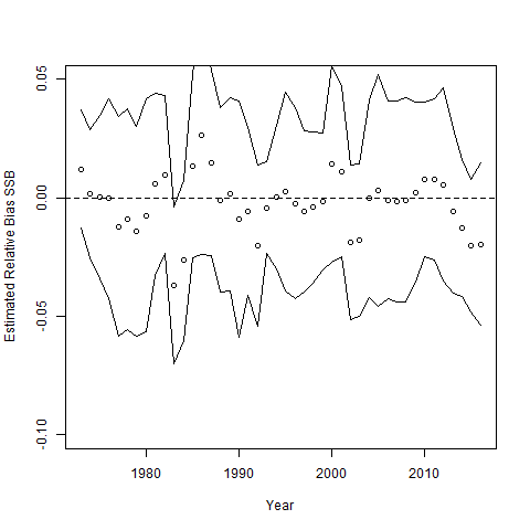
3. Fitting a model different from the operating model
When the fitted model is different from that used to simulate the
data, there is a bit more work involved. Some components of the input
used by fit_wham are important.
input <- prepare_wham_input(
  asap3,
  selectivity = selectivity,
  NAA_re = NAA_re,
  model_name="Ex 1: SNEMA Yellowtail Flounder")
names(input)
#> [1] "data" "par" "map" "years" "years_full"
#> [6] "ages.lab" "model_name" "asap3" "log" "options"
#> [11] "stock_names" "region_names" "fleet_names" "index_names" "years_Ecov"
#> [16] "Ecov_names" "random" "call"Many of the elements of the input (e.g., data,
par, map, random) are those used
by TMB::MakeADFun to set up an objective function with derivative
information (i.e.,gradient, hessian) used by the optimizer nlminb in
fit_wham. We saw above that we could just swap the entire
data element of the input when the estimation model is the
same as the operating model. More generally though, components of these
4 input lists will need to be modified for the simulation studies where
the operating model and estimation model are not the same. If the
available data is the same for the operating and fitted model only a few
elements of the input$data list need to be moved.
3a. An alternative age composition likelihood for the estimating model
Below is an example where an alternative likelihood for the age composition observations is assumed for the estimation model.
input_em <- prepare_wham_input(
  asap3,
  recruit_model=2,
  model_name="Ex 1: SNEMA Yellowtail Flounder",
  selectivity=selectivity,
  NAA_re = NAA_re,
  age_comp = "logistic-normal-miss0") #the only difference from original input

#only eval the observations so that the other inputs for configuration are correct.
#IMPORTANT TO PROVIDE obsvec!
sim_fn = function(om, input, do.fit = FALSE){
  obs_names = c("agg_indices","agg_catch","catch_paa","index_paa", "Ecov_obs", "obsvec")
  om_data = om$simulate(complete = TRUE)
  input$data[obs_names] = om_data[obs_names]
  input <- set_osa_obs(input) #to transform catch and index paa appropriately
  if(do.fit) {
    fit = fit_wham(input, do.sdrep = FALSE, do.osa = FALSE, do.retro = FALSE, MakeADFun.silent = TRUE)
    return(list(fit, om_data))
  } else return(list(input,om_data))
}
By using do.fit = FALSE, we can see the difference between the age composition observations that are fitted and those that were simulated. The 4-9 elements correspond to the index age composition observations in the first year:
set.seed(123)
sim = sim_fn(mod_1, input_em, do.fit = FALSE)
sim[[1]]$data$obs[1:10,] #data.frame of observations and identifying information
sim[[2]]$obsvec[4:9] #showing obsvec that is simulated (multinomial frequencies)
sim[[1]]$data$obsvec[4:9] #showing obsvec that is used (MVN = logistic normal)
paa <- sim[[2]]$index_paa[1,1,]
paa #multinomial proportions : naa/sum(naa)
sim[[2]]$index_Neff[1] * paa # = simulated obsvec (multinomial frequencies)
log(paa[-6]) - log(paa[6]) # = inverse additive logistic transform for obsvec that is used
#> year fleet age type val ind cohort
#> 1 1 index_1 NA logindex 10.4147974 1 NA
#> 2 1 index_2 NA logindex 9.6452466 2 NA
#> 3 1 fleet_1 NA logcatch 9.7927340 3 NA
#> 4 1 index_1 1 indexpaa -0.6931472 4 0
#> 5 1 index_1 2 indexpaa 1.0986123 5 -1
#> 6 1 index_1 3 indexpaa 2.0149030 6 -2
#> 7 1 index_1 4 indexpaa 2.2512918 7 -3
#> 8 1 index_1 5 indexpaa 1.2527630 8 -4
#> 9 1 index_1 6 indexpaa NA 9 -5
#> 10 1 index_2 1 indexpaa 1.3862944 10 0
#> [1] 1 6 15 19 7 2
#> [1] -0.6931472 1.0986123 2.0149030 2.2512918 1.2527630 NA
#> [1] 0.02 0.12 0.30 0.38 0.14 0.04
#> [1] 1 6 15 19 7 2
#> [1] -0.6931472 1.0986123 2.0149030 2.2512918 1.2527630The multinomial was used to simulate the observations and therefore
the observations are frequencies. The logistic normal expects
proportions, but there is an equivalent multivariate normal
transformation that is used to allow the OSA residuals to be calculated
efficiently so this is the form of the observations. Note that the last
age class is NA because the dimension of the MVN is one less than the
number of age classes due to the constraint of proportions summing to 1.
Similarly, the log transform of aggregate index and catch observations
(e.g., first three observations in the obs data.frame above) are
provided in the vector of observations (obsvec) used to fit
the model as those are treated as normal distributed observations.
Now go ahead and fit the simulated data.
set.seed(123)
simfit = sim_fn(mod_1, input_em, do.fit = TRUE)
plot(mod_1$years, simfit[[2]]$SSB, type = 'l', ylab = "SSB", xlab = "Year")
lines(mod_1$years, simfit[[1]]$rep$SSB, lty = 2, col = 'red')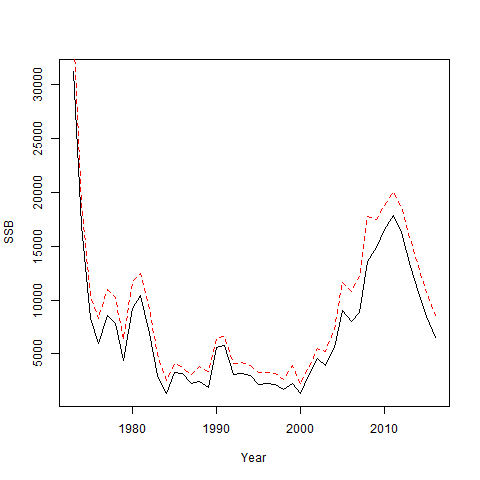
It is very important that the obsvec component of the
simulated data is put into the input used for fitting because this holds
the values in agg_catch, agg_indices, etc. in
vector form for evaluating the likelihood. Having all observations in a
vector is necessary to allow one-step-ahead residuals to be calculated
using the TMB package. Note also because only a few elements are copied
into input$data we need to save all of the true values of
the simulated population as a separate component that is returned. For
this particular simulation, SSB is estimated greater than the truth when
the logistic normal is assumed but observations were generated by a
multinomial. The same sort of approach as above can be used for
simulating and fitting many data sets.
3b. Effective sample size assumption
Suppose we wanted to see how the estimating model behaves when we
assume the multinomial age composition is more precise than it really
is. Here we assume we want to use all of the same parameter estimates
from the original model but change the necessary fixed data inputs. We
modify the input with the appropriate data and populate
input$par with the estimates from the original fit. Then we
create this alternative operating model by calling
fit_wham(input, do.fit=F) which creates the model
configuration with the dll so that data can be simulated with this
particular configuruation. Note that do.fit=F means that
whatever parameter values are set (normally as initial and fixed values)
in input$par will be used to simulate data. For the
estimating model we can use the same input as the operating model except
for changing the inputs for the effective sample size.
sim_fn = function(om, Neff_om = 50, Neff_em = 200, do.fit = FALSE){
  om_input = om$input #the original input
  om_input$data$index_Neff[] = Neff_om #true effective sample size for the indices
  om_input$data$catch_Neff[] = Neff_om #true effective sample size for the indices
  om_input$par = om$parList #as.list(om$sdrep, "Estimate") #assume parameter values estimated from original model
  om_alt = fit_wham(om_input, do.fit = FALSE, MakeADFun.silent=TRUE) #make unfitted model for simulating data
  om_data = om_alt$simulate(complete = TRUE)
  em_input = om_input #the same configuration other than Neff
  em_input$data$index_Neff[] = Neff_em #assumed effective sample size for the indices
  em_input$data$catch_Neff[] = Neff_em #assumed effective sample size for the indices
  obs_names = c("agg_indices","agg_catch","catch_paa","index_paa", "Ecov_obs", "obsvec")
  em_input$data[obs_names] = om_data[obs_names]
  em_input <- set_osa_obs(em_input) #to rescale the frequencies appropriately
  if(do.fit) {
    fit = fit_wham(em_input, do.sdrep = FALSE, do.osa = FALSE, do.retro = FALSE, MakeADFun.silent = TRUE)
    return(list(fit, om_data))
  } else return(list(em_input,om_data))
}
We still need to reset the obsvec because the
frequencies are rescaled by the assumed multinomial sample size. Again,
we can check the observations are being used correctly by usingg do.fit
= FALSE:
set.seed(123)
sim = sim_fn(mod_1, do.fit = FALSE)
sim[[1]]$data$obs[1:10,] #data.frame of observations and identifying information
sim[[2]]$obsvec[4:9] #showing obsvec that is simulated (multinomial frequencies)
sim[[1]]$data$obsvec[4:9] #showing obsvec that is used (MVN = logistic normal)
paa <- sim[[2]]$index_paa[1,1,] #simulated paa
paa #multinomial proportions : naa/sum(naa)
sim[[1]]$data$index_paa[1,1,] #paa in estimating model (the same)
sim[[2]]$index_Neff[1] * paa # = simulated obsvec (multinomial frequencies)
sim[[1]]$data$index_Neff[1] * paa # = em obsvec (multinomial frequencies with larger Neff)
#> year fleet age type val ind cohort
#> 1 1 index_1 NA logindex 10.4147974 1 NA
#> 2 1 index_2 NA logindex 9.6452466 2 NA
#> 3 1 fleet_1 NA logcatch 9.7927340 3 NA
#> 4 1 index_1 1 indexpaa -0.6931472 4 0
#> 5 1 index_1 2 indexpaa 1.0986123 5 -1
#> 6 1 index_1 3 indexpaa 2.0149030 6 -2
#> 7 1 index_1 4 indexpaa 2.2512918 7 -3
#> 8 1 index_1 5 indexpaa 1.2527630 8 -4
#> 9 1 index_1 6 indexpaa NA 9 -5
#> 10 1 index_2 1 indexpaa 1.3862944 10 0
#> [1] 1 6 15 19 7 2
#> [1] -0.6931472 1.0986123 2.0149030 2.2512918 1.2527630 NA
#> [1] 0.02 0.12 0.30 0.38 0.14 0.04
#> [1] 0.02 0.12 0.30 0.38 0.14 0.04
#> [1] 1 6 15 19 7 2
#> [1] 1 6 15 19 7 2We can see that the proportions at age are the same between the operating and estimating model, but the frequencies in the estimating model are 4 times those in the operating model because we are assuming the effective sample size is 4 times the true value.
Now go ahead and fit the simulated data.
set.seed(123)
simfit = sim_fn(mod_1, do.fit = TRUE)

plot(mod_1$years, simfit[[2]]$SSB, type = 'l', ylab = "SSB", xlab = "Year")
lines(mod_1$years, simfit[[1]]$rep$SSB, lty = 2, col = 'red')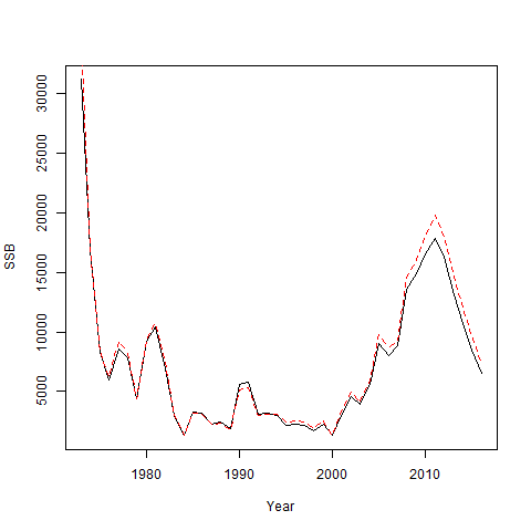
The incorrect age composition precision has a large effect here! Note that we could make the assumed effective sample size only incorrect for some subset of the fleets and indices. Note that changing the Neff will only affect fits to those indices and fleets where the multinomial age comp assumption is made and where age composition observations are available.
3c. Population assumptions
Suppose we wanted to evaluate the effect of assuming a model with just random effects on recruitment when a full state-space model was the operating model. We will fit the full state-space model to the example data to get a configuration for the operating model then simulate data from it and fit the recruitment-only model to it.
NAA_re_om = list(
  sigma="rec+1", #random effects for recruitment and older age classes
  cor="iid", #random effects are independent
  recruit_model = 2) #mean recruitment is the only fixed effect parameter

NAA_re_em = list(
  sigma="rec", #random effects for recruitment only
  cor="iid", #random effects are independent
  recruit_model = 2) #mean recruitment is the only fixed effect parameter

input_om <- prepare_wham_input(
    asap3,
    selectivity = selectivity,
    NAA_re = NAA_re_om,
    model_name="Ex 1: SNEMA Yellowtail Flounder")

input_em <- prepare_wham_input(
    asap3,
    selectivity = selectivity,
    NAA_re = NAA_re_em,
    model_name="Ex 1: SNEMA Yellowtail Flounder")

om_ss <- fit_wham(input_om, do.osa = F, do.retro=F, MakeADFun.silent = T) # don't do retro peels and OSA residuals, don't show output during optimization

#no differences in treatment of observations
sim_fn = function(om, input, do.fit = FALSE){
    obs_names = c("agg_indices","agg_catch","catch_paa","index_paa", "Ecov_obs", "obsvec")
    om_data = om$simulate(complete = TRUE)
    input$data[obs_names] = om_data[obs_names]
    if(do.fit) {
        fit = fit_wham(input, do.sdrep = FALSE, do.osa = FALSE, do.retro = FALSE, MakeADFun.silent = TRUE)
        return(list(fit, om_data))
    } else return(list(input,om_data))
}
set.seed(123)
simfit = sim_fn(om_ss, input_em, do.fit = TRUE)

plot(om_ss$years, simfit[[2]]$SSB, type = 'l', ylab = "SSB", xlab = "Year")
lines(om_ss$years, simfit[[1]]$rep$SSB, lty = 2, col = 'red')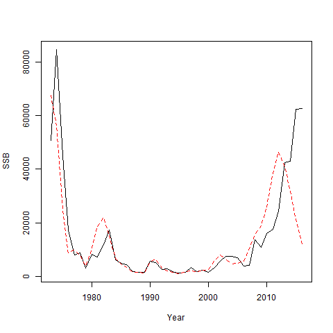
The scale of the population estimates from the recruitment-only model is similar to the true value, but it does not have sufficient flexibility to capture the inter-annual variability in the population size and terminal year stock size is very different.
3d. Selectivity assumptions
Suppose the true selectivity is that estimated from the original
model, but that we wanted to evaluate the effect of assuming logistic
selectivity. Use the same NAA_re defined earlier but change
the selectivity
selectivity_em = list(
  model = c(rep("logistic", input$data$n_fleets),rep("logistic", input$data$n_indices)),
  initial_pars = rep(list(c(5,1)), input$data$n_fleets + input$data$n_indices)) #fleet, index

input_em <- prepare_wham_input(
    asap3,
    selectivity = selectivity_em,
    NAA_re = NAA_re,
    model_name="Ex 1: SNEMA Yellowtail Flounder")

sim_fn = function(om, input, do.fit = FALSE){
    obs_names = c("agg_indices","agg_catch","catch_paa","index_paa", "Ecov_obs", "obsvec")
    om_data = om$simulate(complete = TRUE)
    input$data[obs_names] = om_data[obs_names]
    if(do.fit) {
        fit = fit_wham(input, do.sdrep = FALSE, do.osa = FALSE, do.retro = FALSE, MakeADFun.silent = TRUE)
        return(list(fit, om_data))
    } else return(list(input,om_data))
}
set.seed(123)
simfit = sim_fn(mod_1, input_em, do.fit = TRUE)

plot(mod_1$years, simfit[[2]]$SSB, type = 'l', ylab = "SSB", xlab = "Year")
lines(mod_1$years, simfit[[1]]$rep$SSB, lty = 2, col = 'red')
plot(mod_1$years, simfit[[2]]$SSB/exp(simfit[[2]]$log_SSB_FXSPR[,2]), type = 'l', ylab = "SSB/SSB(F40)", xlab = "Year")
lines(mod_1$years, simfit[[1]]$rep$SSB/exp(simfit[[1]]$rep$log_SSB_FXSPR[,2]), lty = 2, col = 'red')
Lower SSB and stock status are estimated if logistic selectivity is assumed.
4. Creating a general operating model without an ASAP3 dat file
Note that the simulated data are conditioned on the fixed effects
parameter values. If a model is fitted using fit_wham then
the optimized values will be used by mod$simulate for
simulations, but these parameters can be specified without fitting the
model and simulations can be more generally configured. Here we will use
the functionality of prepare_wham_input to create a model
object without an asap3 dat file and, then set parameter values we want
to assume for the operating model
First we will read in a function make_info that will
make a list that can be provided to the basic_info ,
catch_info, and index_info arguments of
prepare_wham_input. The elements of the output it provides
are defined in the help file for prepare_wham_input.
make_info <- function(base_years = 1982:2021, ages = 1:10, Fhist = "updown", n_feedback_years = 0) { #changed years
    info <- list()
    info$ages <- ages
    info$years <- as.integer(base_years[1] - 1 + 1:(length(base_years) + n_feedback_years))
    na <- length(info$ages)
    ny <- length(info$years)
    info$n_regions <- 1L
    info$n_stocks <- 1L
    nby <- length(base_years)
    mid <- floor(nby/2)
    #up then down

    catch_info <- list()
    catch_info$n_fleets <- 1L
    catch_info$catch_cv <- matrix(0.1, ny, catch_info$n_fleets)
    catch_info$catch_Neff <- matrix(200, ny, catch_info$n_fleets)

    F_info <- list()
    if(Fhist == "updown") F_info$F <- matrix(0.2 + c(seq(0,0.4,length.out = mid),seq(0.4,0,length.out=nby-mid)),nby, catch_info$n_fleets)

    #down then up
    if(Fhist == "downup") F_info$F <- matrix(0.2 + c(seq(0.4,0,length.out = mid),seq(0,0.4,length.out=nby-mid)),nby, catch_info$n_fleets)

    if(n_feedback_years>0) F_info$F <- rbind(F_info$F, F_info$F[rep(nby, n_feedback_years),, drop = F]) #same F as terminal year for feedback period

    index_info <- list()
    index_info$n_indices <- 1L
    index_info$index_cv <- matrix(0.3, ny, index_info$n_indices)
    index_info$index_Neff <- matrix(100, ny, index_info$n_indices)
    index_info$fracyr_indices <- matrix(0.5, ny, index_info$n_indices)
    index_info$units_index <- rep(1, length(index_info$n_indices)) #biomass
    index_info$units_index_paa <- rep(2, length(index_info$n_indices)) #abundance
    index_info$q <- rep(0.3, index_info$n_indices)

    info$maturity <- array(t(matrix(1/(1 + exp(-1*(1:na - na/2))), na, ny)), dim = c(1, ny, na))

    L <- 100*(1-exp(-0.3*(1:na - 0)))
    W <- exp(-11)*L^3
    nwaa <- index_info$n_indices + catch_info$n_fleets + 2
    info$waa <- array(NA, dim = c(nwaa, ny, na))
    for(i in 1:nwaa) info$waa[i,,] <- t(matrix(W, na, ny))

    info$fracyr_SSB <- cbind(rep(0.25,ny))

    catch_info$selblock_pointer_fleets <- t(matrix(1:catch_info$n_fleets, catch_info$n_fleets, ny))
    index_info$selblock_pointer_indices <- t(matrix(catch_info$n_fleets + 1:index_info$n_indices, index_info$n_indices, ny))
    return(list(basic_info = info, catch_info = catch_info, index_info = index_info, F = F_info))
}
Various attributes are specified in the make_info
function including the number of fleets and indices, the years over
which the model spans, the number of ages, precision of aggregate catch
and index observations. Maturity and weight at age are defined as well
as catchabilities for the indices, when they occur during the year and
the selectivity blocks to assign to each fleet and index. The function
creates a list of four lists that are arguments to
prepare_wham_input: basic_info,
catch_info, index_info, and F.
The potential elements that might be supplied to these arguments are
described in the help files for prepare_wham_input and
helper functions set_*.
Many other necessary attributes and initial parameters can be defined
using the arguments NAA_re, selectivity,
M, catchability, or move (when
there is more than 1 region) to prepare_wham_input. Below
we specify logistic selectivity and associated parameters
(
and slope), M = 0.2, initial numbers at age, and mean recruitment all
using the lists supplied to these arguments of prepare_wham_input. We
also specify a value for the standard deviation of the (log) recruitment
random effects
().
Importantly, fit_wham must be called with
do.fit=FALSE to set up the model to be simulated with the
parameter values specified rather than estimated.
stock_om_info <- make_info()
basic_info <- stock_om_info$basic_info
catch_info <- stock_om_info$catch_info
index_info <- stock_om_info$index_info
F_info <- stock_om_info$F

selectivity_om <- list(
  model = c(rep("logistic", catch_info$n_fleets),rep("logistic", index_info$n_indices)),
  initial_pars = rep(list(c(5,1)), catch_info$n_fleets + index_info$n_indices)
) #fleet, index

M_om <- list(initial_means = array(0.2, dim = c(1,1, length(basic_info$ages))))

NAA_re_om <- list(
  N1_pars = array(exp(10)*exp(-(0:(length(basic_info$ages)-1))*M_om$initial_means[1]), dim = c(1,1,length(basic_info$ages))),
  sigma = "rec", #random about mean
  cor="iid", #random effects are independent
  recruit_model = 2, #random effects with a constant mean
  recruit_pars = list(exp(10)),
  sigma_vals = array(0.5, c(1,1,length(basic_info$ages))) #sigma_R, only the value in the first age class is used.
)

stock_om_input <- prepare_wham_input(
  basic_info = basic_info,
  selectivity = selectivity_om,
  NAA_re = NAA_re_om,
  catch_info = catch_info,
  index_info = index_info,
  M = M_om,
    F = F_info
)
#>
#> --Creating input---------------------------------------------------------------------------------------------------------------------
#> basic_info done
#> catch done
#> indices done
#> WAA done
#> NAA done
#> q done
#> selectivity done
#> age_comp done
#> F done
#> M done
#> move done
#> osa_obs done
#> --Input Complete--------------------------------------------------------------------------------------------------------------------
#> -------------------------------------------------------------------------------------------------------------------------------------
#> WHAM version 2.0.0 and forward:
#> 1) makes major changes to the structure of some data, parameters, and reported objects.
#> 2) decouples random effects for recruitment and random effects for older ages by default. To obtain results from previous versions set NAA_re$decouple_recruitment = FALSE.
#> 3) does not bias correct any log-normal process or observation errors. To configure these, set basic_info$bias_correct_process = TRUE and/or basic_info$bias_correct_observation = TRUE.
#> -------------------------------------------------------------------------------------------------------------------------------------
#> input$data$spawn_regions will be defined from input$data$NAA_where for age 1.
#> --Catch------------------------------------------------------------------------------------------------------------------------------
#> catch_info$waa_pointer_fleets was not provided, so the first waa matrix will be used for all fleets.
#> Selectivity blocks for each fleet:
#> Fleet 1: 1
#>
#> -------------------------------------------------------------------------------------------------------------------------------------
#>
#> --Indices----------------------------------------------------------------------------------------------------------------------------
#> Selectivity blocks for each index:
#> index_1: 2
#>
#> -------------------------------------------------------------------------------------------------------------------------------------
#>
#> --WAA--------------------------------------------------------------------------------------------------------------------------------
#> basic_info$waa_pointer_ssb was not provided and no asap3 file(s), so the first waa matrix will be used.
#> basic_info$waa_pointer_M was not provided, so waa_pointer_ssb will be used.
#> -------------------------------------------------------------------------------------------------------------------------------------
#>
#> --NAA--------------------------------------------------------------------------------------------------------------------------------
#>
#>  Same NAA_re$sigma being used for all stocks (rec).
#> -------------------------------------------------------------------------------------------------------------------------------------
#>
#> --Selectivity------------------------------------------------------------------------------------------------------------------------
#> selectivity$n_selblocks was not provided so number of selblocks: 2, is being determined by max(input$data$selblock_pointer_fleets,input$data$selblock_pointer_indices).
#> (Mean) selectivity block models are:
#> Block 1: logistic
#> Block 2: logistic
#>
#> Random effects options for each selectivity block are:
#> Block 1: none
#> Block 2: none
#>
#> -------------------------------------------------------------------------------------------------------------------------------------
#>
#> --Reference points-------------------------------------------------------------------------------------------------------------------
#> For annual SPR-based reference points, corresponding annual conditionally expected recruitments are used.
#> -------------------------------------------------------------------------------------------------------------------------------------

#stock_om <- fit_wham(stock_om_input, do.fit = FALSE, MakeADFun.silent = TRUE)
#n_stock x n_regions x n_ages array
exp(stock_om_input$par$log_NAA_sigma[1,1,1]) #Rsigma
#> [1] 0.5
4a. Setting NAA random effects variance parameters.
Here we will consider a 2d AR1 autoregressing model for the numbers
at age random effects to demonstrate setting the parameters. We will
suppose that we want to assume (or initialize) standard deviations of
0.6 for recruitment and 0.2 for older ages. When random effects are
assumed for both recruitment and survival transitions of older age
classes, wham now decouples these two types of random effects so they
are independent. We will assume correlation of 0.7 with age for age
greater than recruitment and correlations of 0.4 and 0.6, temporally,
for survival transitions and recruitment, respectively. There are two
parameter elements that we need to consider when using these random
effects: log_NAA_sigma as mentioned above and
trans_NAA_rho which defines the autocorrelation parameters
on a logit scale with the parameter bounds of (-1,1). These parameters
can be set using the NAA_re argument to
prepare_wham_input. See the help file for
set_NAA.
NAA_re_om <- list(
  N1_pars = array(exp(10)*exp(-(0:(length(basic_info$ages)-1))*M_om$initial_means[1]), dim = c(1,1,length(basic_info$ages))),
  sigma = "rec+1", #random about mean
  cor="2dar1", #random effects correlated among age classes and across time (separably)
  recruit_model = 2, #random effects with a constant mean
  decouple_recruitment = TRUE, #default value
  recruit_pars = list(exp(10)),
  sigma_vals = array(c(0.6, rep(0.2,length(basic_info$ages)-1)), c(1,1,length(basic_info$ages))), #sigma_R and sigma_2+
  cor_vals = array(c(0.7, 0.4, 0.6), c(1,1,3)) #age, then year (2+, then recruitment)
)

stock_om_input <- prepare_wham_input(
  basic_info = basic_info,
  selectivity = selectivity_om,
  NAA_re = NAA_re_om,
  catch_info = catch_info,
  index_info = index_info,
  M = M_om,
    F = F_info
)
#>
#> --Creating input---------------------------------------------------------------------------------------------------------------------
#> basic_info done
#> catch done
#> indices done
#> WAA done
#> NAA done
#> q done
#> selectivity done
#> age_comp done
#> F done
#> M done
#> move done
#> osa_obs done
#> --Input Complete--------------------------------------------------------------------------------------------------------------------
#> -------------------------------------------------------------------------------------------------------------------------------------
#> WHAM version 2.0.0 and forward:
#> 1) makes major changes to the structure of some data, parameters, and reported objects.
#> 2) decouples random effects for recruitment and random effects for older ages by default. To obtain results from previous versions set NAA_re$decouple_recruitment = FALSE.
#> 3) does not bias correct any log-normal process or observation errors. To configure these, set basic_info$bias_correct_process = TRUE and/or basic_info$bias_correct_observation = TRUE.
#> -------------------------------------------------------------------------------------------------------------------------------------
#> input$data$spawn_regions will be defined from input$data$NAA_where for age 1.
#> --Catch------------------------------------------------------------------------------------------------------------------------------
#> catch_info$waa_pointer_fleets was not provided, so the first waa matrix will be used for all fleets.
#> Selectivity blocks for each fleet:
#> Fleet 1: 1
#>
#> -------------------------------------------------------------------------------------------------------------------------------------
#>
#> --Indices----------------------------------------------------------------------------------------------------------------------------
#> Selectivity blocks for each index:
#> index_1: 2
#>
#> -------------------------------------------------------------------------------------------------------------------------------------
#>
#> --WAA--------------------------------------------------------------------------------------------------------------------------------
#> basic_info$waa_pointer_ssb was not provided and no asap3 file(s), so the first waa matrix will be used.
#> basic_info$waa_pointer_M was not provided, so waa_pointer_ssb will be used.
#> -------------------------------------------------------------------------------------------------------------------------------------
#>
#> --NAA--------------------------------------------------------------------------------------------------------------------------------
#>
#>  Same NAA_re$sigma being used for all stocks (rec+1).
#> -------------------------------------------------------------------------------------------------------------------------------------
#>
#> --Selectivity------------------------------------------------------------------------------------------------------------------------
#> selectivity$n_selblocks was not provided so number of selblocks: 2, is being determined by max(input$data$selblock_pointer_fleets,input$data$selblock_pointer_indices).
#> (Mean) selectivity block models are:
#> Block 1: logistic
#> Block 2: logistic
#>
#> Random effects options for each selectivity block are:
#> Block 1: none
#> Block 2: none
#>
#> -------------------------------------------------------------------------------------------------------------------------------------
#>
#> --Reference points-------------------------------------------------------------------------------------------------------------------
#> For annual SPR-based reference points, corresponding annual conditionally expected recruitments are used.
#> -------------------------------------------------------------------------------------------------------------------------------------

#or equivalently
#stock_om_input <- set_NAA(stock_om_input, NAA_re_om)
#n_stock x n_regions x 3 array
stock_om_input$par$trans_NAA_rho[1,1,1:3]
#> [1] 1.7346011 0.8472979 1.3862944
wham:::gen.logit(c(0.7,0.4,0.6), -1, 1) #age first, year (2+) second, year (rec) third
#> [1] 1.7346011 0.8472979 1.3862944
Note we made use of an unexported function from the wham package that
can do the transformation of parameters estimated on the logit scale.
Note also, that the correlation parameter for age is first and those for
time are second and third in the trans_NAA_rho vector. If
cor = 'ar1_a' only the first parameter in
trans_NAA_rho is used and if cor = 'ar1_y'
only the second and third parameters are used. Other values are set to
zero automatically so the random effects independent in the appropriate
way. Now if we built the operating model:
stock_om <- fit_wham(stock_om_input, do.fit = FALSE, MakeADFun.silent = TRUE)calling stock_om$simulate() will use the variance anc
correlation as we specified.
4b. Setting M random effects variance parameters
M random effects assumptions are similar to the NAA random effects,
but the parameter names are different. For M there is an array (n_stocks
x n_regions x 3) M_repars of values that define the
transformed M variance and autoregressing parameters. for a given stock
and region, the three parameters are standard deviation, correlation
with age, correlation with year. Here we assume we have random effects
on recruitment and on natural mortality. As above, we define the general
model to have 2dAR1 for M random effects for the most general case with
variance of the (log) M random effects = 0.1 and correlations with age
and time of 0.7 and 0.4. However, we can use the M argument
to prepare_wham_input to specify many of these
configurations. See the help file for set_M.
M_om <- list(
  re_model = matrix("ar1_ay", 1,1),
    initial_means = array(0.2, dim = c(1,1, length(basic_info$ages))),
    sigma_vals = matrix(0.2, 1,1),
    cor_vals = array(c(0.7,0.4),dim = c(1,1,2)))

NAA_re_om <- list(
  N1_pars = array(exp(10)*exp(-(0:(length(basic_info$ages)-1))*M_om$initial_means[1]), dim = c(1,1,length(basic_info$ages))),
  sigma = "rec", #random about mean
  recruit_model = 2, #random effects with a constant mean
  sigma_vals = array(0.6, c(1,1,length(basic_info$ages))), #sigma_R
  recruit_pars = list(exp(10))
)

stock_om_input <- prepare_wham_input(
  basic_info = basic_info,
  selectivity = selectivity_om,
  NAA_re = NAA_re_om,
  catch_info = catch_info,
  index_info = index_info,
  M = M_om,
    F = F_info
)
#>
#> --Creating input---------------------------------------------------------------------------------------------------------------------
#> basic_info done
#> catch done
#> indices done
#> WAA done
#> NAA done
#> q done
#> selectivity done
#> age_comp done
#> F done
#> M done
#> move done
#> osa_obs done
#> --Input Complete--------------------------------------------------------------------------------------------------------------------
#> -------------------------------------------------------------------------------------------------------------------------------------
#> WHAM version 2.0.0 and forward:
#> 1) makes major changes to the structure of some data, parameters, and reported objects.
#> 2) decouples random effects for recruitment and random effects for older ages by default. To obtain results from previous versions set NAA_re$decouple_recruitment = FALSE.
#> 3) does not bias correct any log-normal process or observation errors. To configure these, set basic_info$bias_correct_process = TRUE and/or basic_info$bias_correct_observation = TRUE.
#> -------------------------------------------------------------------------------------------------------------------------------------
#> input$data$spawn_regions will be defined from input$data$NAA_where for age 1.
#> --Catch------------------------------------------------------------------------------------------------------------------------------
#> catch_info$waa_pointer_fleets was not provided, so the first waa matrix will be used for all fleets.
#> Selectivity blocks for each fleet:
#> Fleet 1: 1
#>
#> -------------------------------------------------------------------------------------------------------------------------------------
#>
#> --Indices----------------------------------------------------------------------------------------------------------------------------
#> Selectivity blocks for each index:
#> index_1: 2
#>
#> -------------------------------------------------------------------------------------------------------------------------------------
#>
#> --WAA--------------------------------------------------------------------------------------------------------------------------------
#> basic_info$waa_pointer_ssb was not provided and no asap3 file(s), so the first waa matrix will be used.
#> basic_info$waa_pointer_M was not provided, so waa_pointer_ssb will be used.
#> -------------------------------------------------------------------------------------------------------------------------------------
#>
#> --NAA--------------------------------------------------------------------------------------------------------------------------------
#>
#>  Same NAA_re$sigma being used for all stocks (rec).
#> -------------------------------------------------------------------------------------------------------------------------------------
#>
#> --Selectivity------------------------------------------------------------------------------------------------------------------------
#> selectivity$n_selblocks was not provided so number of selblocks: 2, is being determined by max(input$data$selblock_pointer_fleets,input$data$selblock_pointer_indices).
#> (Mean) selectivity block models are:
#> Block 1: logistic
#> Block 2: logistic
#>
#> Random effects options for each selectivity block are:
#> Block 1: none
#> Block 2: none
#>
#> -------------------------------------------------------------------------------------------------------------------------------------
#>
#> --Reference points-------------------------------------------------------------------------------------------------------------------
#> For annual SPR-based reference points, corresponding annual conditionally expected recruitments are used.
#> -------------------------------------------------------------------------------------------------------------------------------------


#or equivalently
#stock_om_input <- set_NAA(stock_om_input, NAA_re_om)
#stock_om_input <- set_M(stock_om_input, M_om)
#n_stock x n_regions x 3 array

exp(stock_om_input$par$log_NAA_sigma[1,1,1]) #Rsigma
#> [1] 0.6

exp(stock_om_input$par$M_repars[1,1,1]) #
#> [1] 0.2

stock_om_input$par$M_repars[1,1,2:3]
#> [1] 1.7346011 0.8472979
wham:::gen.logit(c(0.7,0.4), -1, 1) #age first, year second
#> [1] 1.7346011 0.8472979

#stock_om = fit_wham(stock_om_input, do.fit = FALSE, MakeADFun.silent = TRUE)
Note that the initial values for the mean of the M autoregressing
random effects is defined by the initial_means component of
the M argument to prepare_wham_input. These
mean parameters are not estimated by default, and so therefore are fixed
at these initial values. To estimate the mean of the M random effects at
age, or just estimate a constant M without random effects, specify
M$mean_model = "estimate-M". The default is to estimate a
single value for each stock, but to estimates different mean parameters
across age (and possibly stock and region) specify
M$means_map as an array (n_stock x n_regions x n_ages)
where shared parameters (e.g., all ages) should have the same value.
There is a difference from numbers at age in how random effects for M
are specified. If M$re = "ar_a", then there are only
n_ages random effects that are constant over time.
Similarly for M$re = "ar_y", there are
n_years_model random effects that are used for each age
class. Setting the variance and correlation parameters is similar to
that for numbers at age random effects. To get ar_a or
ar_y models analogous to numbers at age, one would have to
specify M$re = "2dar1" and set M$cor_map to
fix the appropriate parameter fixed at 0. To force random effects for
certain age classes to be the same, one can configure
M$re_map appropriately.
M_om <- list(
  mean_model = "estimate-M",
  re_model = matrix("ar1_ay", 1,1),
    initial_means = array(0.2, dim = c(1,1, length(basic_info$ages))),
    #means_map = array(1, dim(c(1,1,, length(basic_info$ages)))), #one parameters for all ages (the default)
    sigma_vals = matrix(0.2, 1,1),
    cor_vals = array(c(0.7,0.4),dim = c(1,1,2)))

stock_om_input <- prepare_wham_input(
  basic_info = basic_info,
  selectivity = selectivity_om,
  NAA_re = NAA_re_om,
  catch_info = catch_info,
  index_info = index_info,
  M = M_om,
    F = F_info
)
#>
#> --Creating input---------------------------------------------------------------------------------------------------------------------
#> basic_info done
#> catch done
#> indices done
#> WAA done
#> NAA done
#> q done
#> selectivity done
#> age_comp done
#> F done
#> M done
#> move done
#> osa_obs done
#> --Input Complete--------------------------------------------------------------------------------------------------------------------
#> -------------------------------------------------------------------------------------------------------------------------------------
#> WHAM version 2.0.0 and forward:
#> 1) makes major changes to the structure of some data, parameters, and reported objects.
#> 2) decouples random effects for recruitment and random effects for older ages by default. To obtain results from previous versions set NAA_re$decouple_recruitment = FALSE.
#> 3) does not bias correct any log-normal process or observation errors. To configure these, set basic_info$bias_correct_process = TRUE and/or basic_info$bias_correct_observation = TRUE.
#> -------------------------------------------------------------------------------------------------------------------------------------
#> input$data$spawn_regions will be defined from input$data$NAA_where for age 1.
#> --Catch------------------------------------------------------------------------------------------------------------------------------
#> catch_info$waa_pointer_fleets was not provided, so the first waa matrix will be used for all fleets.
#> Selectivity blocks for each fleet:
#> Fleet 1: 1
#>
#> -------------------------------------------------------------------------------------------------------------------------------------
#>
#> --Indices----------------------------------------------------------------------------------------------------------------------------
#> Selectivity blocks for each index:
#> index_1: 2
#>
#> -------------------------------------------------------------------------------------------------------------------------------------
#>
#> --WAA--------------------------------------------------------------------------------------------------------------------------------
#> basic_info$waa_pointer_ssb was not provided and no asap3 file(s), so the first waa matrix will be used.
#> basic_info$waa_pointer_M was not provided, so waa_pointer_ssb will be used.
#> -------------------------------------------------------------------------------------------------------------------------------------
#>
#> --NAA--------------------------------------------------------------------------------------------------------------------------------
#>
#>  Same NAA_re$sigma being used for all stocks (rec).
#> -------------------------------------------------------------------------------------------------------------------------------------
#>
#> --Selectivity------------------------------------------------------------------------------------------------------------------------
#> selectivity$n_selblocks was not provided so number of selblocks: 2, is being determined by max(input$data$selblock_pointer_fleets,input$data$selblock_pointer_indices).
#> (Mean) selectivity block models are:
#> Block 1: logistic
#> Block 2: logistic
#>
#> Random effects options for each selectivity block are:
#> Block 1: none
#> Block 2: none
#>
#> -------------------------------------------------------------------------------------------------------------------------------------
#>
#> --Reference points-------------------------------------------------------------------------------------------------------------------
#> For annual SPR-based reference points, corresponding annual conditionally expected recruitments are used.
#> -------------------------------------------------------------------------------------------------------------------------------------


#or equivalently
#stock_om_input <- set_M(stock_om_input, M_om)
stock_om_input$map$Mpars
4c. Setting selectivity random effects variance parameters
Setting the variance parameters for selectivity random effects is
analogous to that for natural mortality random effects. The important
difference is that the parameter object defining the random effects
variance parameters (sel_repars) is a matrix with rows for
each selectivity block and the 3 columns as defined for
M_repars. Here we have two selectivity blocks: one for the
fleet and one for the index. We will assume that the variance parameter
for the fleet is 0.4 and that for the index is 0.1, but they both have
the same correlation parameters with age and time: 0.7 and 0.4. See the
help file for set_selectivity.
selectivity_om = list(
  model = c(rep("logistic", catch_info$n_fleets),rep("logistic", index_info$n_indices)),
  initial_pars = rep(list(c(5,1)), catch_info$n_fleets + index_info$n_indices),
  re = rep("2dar1", catch_info$n_fleets + index_info$n_indices),
  sigma_vals = c(0.4,0.1),
  cor_vals = cbind(rep(0.7,2),rep(0.4,2))
)

#remove random effects on M
M_om <- list(
  initial_means = array(0.2, dim = c(1,1, length(basic_info$ages)))
)

stock_om_input <- prepare_wham_input(
  basic_info = basic_info,
  selectivity = selectivity_om,
  NAA_re = NAA_re_om,
  catch_info = catch_info,
  index_info = index_info,
  M = M_om,
    F = F_info
)
#>
#> --Creating input---------------------------------------------------------------------------------------------------------------------
#> basic_info done
#> catch done
#> indices done
#> WAA done
#> NAA done
#> q done
#> selectivity done
#> age_comp done
#> F done
#> M done
#> move done
#> osa_obs done
#> --Input Complete--------------------------------------------------------------------------------------------------------------------
#> -------------------------------------------------------------------------------------------------------------------------------------
#> WHAM version 2.0.0 and forward:
#> 1) makes major changes to the structure of some data, parameters, and reported objects.
#> 2) decouples random effects for recruitment and random effects for older ages by default. To obtain results from previous versions set NAA_re$decouple_recruitment = FALSE.
#> 3) does not bias correct any log-normal process or observation errors. To configure these, set basic_info$bias_correct_process = TRUE and/or basic_info$bias_correct_observation = TRUE.
#> -------------------------------------------------------------------------------------------------------------------------------------
#> input$data$spawn_regions will be defined from input$data$NAA_where for age 1.
#> --Catch------------------------------------------------------------------------------------------------------------------------------
#> catch_info$waa_pointer_fleets was not provided, so the first waa matrix will be used for all fleets.
#> Selectivity blocks for each fleet:
#> Fleet 1: 1
#>
#> -------------------------------------------------------------------------------------------------------------------------------------
#>
#> --Indices----------------------------------------------------------------------------------------------------------------------------
#> Selectivity blocks for each index:
#> index_1: 2
#>
#> -------------------------------------------------------------------------------------------------------------------------------------
#>
#> --WAA--------------------------------------------------------------------------------------------------------------------------------
#> basic_info$waa_pointer_ssb was not provided and no asap3 file(s), so the first waa matrix will be used.
#> basic_info$waa_pointer_M was not provided, so waa_pointer_ssb will be used.
#> -------------------------------------------------------------------------------------------------------------------------------------
#>
#> --NAA--------------------------------------------------------------------------------------------------------------------------------
#>
#>  Same NAA_re$sigma being used for all stocks (rec).
#> -------------------------------------------------------------------------------------------------------------------------------------
#>
#> --Selectivity------------------------------------------------------------------------------------------------------------------------
#> selectivity$n_selblocks was not provided so number of selblocks: 2, is being determined by max(input$data$selblock_pointer_fleets,input$data$selblock_pointer_indices).
#> (Mean) selectivity block models are:
#> Block 1: logistic
#> Block 2: logistic
#>
#> Random effects options for each selectivity block are:
#> Block 1: 2dar1
#> Block 2: 2dar1
#>
#> -------------------------------------------------------------------------------------------------------------------------------------
#>
#> --Reference points-------------------------------------------------------------------------------------------------------------------
#> For annual SPR-based reference points, corresponding annual conditionally expected recruitments are used.
#> -------------------------------------------------------------------------------------------------------------------------------------


#or equivalently
#stock_om_input <- set_M(stock_om_input, M_om)
#stock_om_input <- set_selectivity(stock_om_input, selectivity_om)
stock_om_input$par$sel_repars
#>            [,1]     [,2]      [,3]
#> [1,] -0.9162907 1.734601 0.8472979
#> [2,] -2.3025851 1.734601 0.8472979
rbind(c(log(0.4), wham:::gen.logit(c(0.7,0.4),-1,1)),
c(log(0.1), wham:::gen.logit(c(0.7,0.4),-1,1)))
#>            [,1]     [,2]      [,3]
#> [1,] -0.9162907 1.734601 0.8472979
#> [2,] -2.3025851 1.734601 0.8472979
Note in this case where we assume logistic selectivity and 2D AR1
random effects, the correlation with “age” is actually just the
correlation of the two logistic selectivity parameters on their
estimated/transformed scale. Also, differing from natural mortality the
mean parameters for the selectivity random effects
(logit_selpars) are estimated by default.
4d. Setting catchability random effects variance parameters.
Setting the variance parameters for catchability is analogous to that
for natural mortality and selectivity random effects. The parameters
defining the variance and correlation of the annual catchability are
defined in q_repars which is a matrix with rows
corresponding to different indices and 2 columns for the standard
deviation and correlation. The mean of the process is defined and
estimated in the logit_q parameter which is defined in the
make_basic_info function. Here we will assume the
transformed catchability is an AR1 process with standard deviation 0.1
and autocorrelation = 0.5.
selectivity_om = list(
  model = c(rep("logistic", catch_info$n_fleets),rep("logistic", index_info$n_indices)),
  initial_pars = rep(list(c(5,1)), catch_info$n_fleets + index_info$n_indices)
)

catchability_om = list(
    re = "ar1",
    sigma_vals = 0.1,
    cor_vals = 0.5) #could also define the mean q parameter here.

stock_om_input <- prepare_wham_input(
  basic_info = basic_info,
  selectivity = selectivity_om,
  NAA_re = NAA_re_om,
  catch_info = catch_info,
  index_info = index_info,
  catchability = catchability_om,
  M = M_om,
    F = F_info
)
#>
#> --Creating input---------------------------------------------------------------------------------------------------------------------
#> basic_info done
#> catch done
#> indices done
#> WAA done
#> NAA done
#> q done
#> selectivity done
#> age_comp done
#> F done
#> M done
#> move done
#> osa_obs done
#> --Input Complete--------------------------------------------------------------------------------------------------------------------
#> -------------------------------------------------------------------------------------------------------------------------------------
#> WHAM version 2.0.0 and forward:
#> 1) makes major changes to the structure of some data, parameters, and reported objects.
#> 2) decouples random effects for recruitment and random effects for older ages by default. To obtain results from previous versions set NAA_re$decouple_recruitment = FALSE.
#> 3) does not bias correct any log-normal process or observation errors. To configure these, set basic_info$bias_correct_process = TRUE and/or basic_info$bias_correct_observation = TRUE.
#> -------------------------------------------------------------------------------------------------------------------------------------
#> input$data$spawn_regions will be defined from input$data$NAA_where for age 1.
#> --Catch------------------------------------------------------------------------------------------------------------------------------
#> catch_info$waa_pointer_fleets was not provided, so the first waa matrix will be used for all fleets.
#> Selectivity blocks for each fleet:
#> Fleet 1: 1
#>
#> -------------------------------------------------------------------------------------------------------------------------------------
#>
#> --Indices----------------------------------------------------------------------------------------------------------------------------
#> Selectivity blocks for each index:
#> index_1: 2
#>
#> -------------------------------------------------------------------------------------------------------------------------------------
#>
#> --WAA--------------------------------------------------------------------------------------------------------------------------------
#> basic_info$waa_pointer_ssb was not provided and no asap3 file(s), so the first waa matrix will be used.
#> basic_info$waa_pointer_M was not provided, so waa_pointer_ssb will be used.
#> -------------------------------------------------------------------------------------------------------------------------------------
#>
#> --NAA--------------------------------------------------------------------------------------------------------------------------------
#>
#>  Same NAA_re$sigma being used for all stocks (rec).
#> -------------------------------------------------------------------------------------------------------------------------------------
#>
#> --Selectivity------------------------------------------------------------------------------------------------------------------------
#> selectivity$n_selblocks was not provided so number of selblocks: 2, is being determined by max(input$data$selblock_pointer_fleets,input$data$selblock_pointer_indices).
#> (Mean) selectivity block models are:
#> Block 1: logistic
#> Block 2: logistic
#>
#> Random effects options for each selectivity block are:
#> Block 1: none
#> Block 2: none
#>
#> -------------------------------------------------------------------------------------------------------------------------------------
#>
#> --Reference points-------------------------------------------------------------------------------------------------------------------
#> For annual SPR-based reference points, corresponding annual conditionally expected recruitments are used.
#> -------------------------------------------------------------------------------------------------------------------------------------


#or equivalently
#stock_om_input <- set_selectivity(stock_om_input, selectivity_om)
#stock_om_input <- set_q(stock_om_input, catchability_om)
stock_om_input$par$q_repars
#>           [,1]     [,2]
#> [1,] -2.302585 1.098612
c(log(0.1), wham:::gen.logit(0.5,-1,1))
#> [1] -2.302585  1.098612
stock_om = fit_wham(stock_om_input, do.fit = FALSE, MakeADFun.silent = TRUE)

set.seed(123)
sim_q = stock_om$simulate(complete=TRUE)

plot(stock_om$years, sim_q$q[,1], type = 'l', ylab = "Catchability", xlab = "Year")
4e. Setting effects of environmental covariates.
When environmental effects are considered, there are assumptions to
be made about the variance and any autocorrelation parameters for the
random effects for the latent environmental process and the variance of
the observation errors. The latter are specified in the the
ecov$log_sigma argument to prepare_wham_input
and those for the random effects (Ecov_process_pars) are
specified the ecov$process_mean_vals,
ecov$process_sig_vals, and
ecov$process_cor_vals arguments. The value for the effect
of the covariate on recruitment (Ecov_beta_R) are specified
in ecov$beta_R_vals. The columns of
Ecov_process_pars correspond to each environmental
covariate being modeled and the number of rows is 3. If
ecov$process_model = "rw" only the first two elements are
used and represent the value in the first year and the conditional
standard deviation parameter of the random walk. When
ecov$process_model = "ar1" the three elements correspond to
mean, variance, and correlation parameters.
The Ecov_beta parameter is a 4-dimensional array to be
able to use it across all possible types of effects in a wham model. The
first dimension indicates where the effect will be applied: recruitment,
natural mortality, index 1,… index n. The second dimension is the order
of the polynomial effect of the covariate. The third dimension indicates
which environmental covariate the effect is having on the population.
The fourth dimension indicates which age class the effect is on (for
natural mortality only).
As long as there is only a single environmental effect, we can change
the appropriate element of the Ecov_beta array by using the
map$Ecov_beta specification returned by
prepare_wham_input. The map$Ecov_beta will be
all NA except for the configured effects on the population
and when there is just one there is no ambiguity. Otherwise, the 4
correct indices of the Ecov_beta array must be referenced
appropriately for each effect.
We will assume that our errors on the observations of the
environmental covariate have a standard deviation = 0.2, the latent
process is AR1 with mean 0, standard deviation = 0.3 and correlation
parameter 0.5. We will also assume the effect is on (log) recruitment
(no stock-recruit function) and the size of the effect is
Ecov_beta = 0.3.
ecov_om = list(
    label = "Climate variable 1",
    process_model = "ar1",
    process_mean_vals = 0,
    process_sig_vals = 0.3,
    process_cor_vals = 0.5,
    mean = matrix(0, length(basic_info$years), 1), #observations which will be simulated later
    logsigma = log(0.2),
    year = basic_info$years,
    use_obs = matrix(1,length(basic_info$years),1),
    recruitment_how = matrix("controlling-lag-0-linear",1,1),
    beta_R_vals = array(0.3, dim = c(1,1,1))
 )

stock_om_input = prepare_wham_input(
    basic_info = basic_info,
    selectivity = selectivity_om,
    NAA_re = NAA_re_om,
    M = M_om,
  catch_info = catch_info,
  index_info = index_info,
    ecov = ecov_om,
    F = F_info
)
#>
#> --Creating input---------------------------------------------------------------------------------------------------------------------
#> basic_info done
#> catch done
#> indices done
#> WAA done
#> NAA done
#> q done
#> selectivity done
#> age_comp done
#> F done
#> M done
#> move done
#> ecov done
#> osa_obs done
#> --Input Complete--------------------------------------------------------------------------------------------------------------------
#> -------------------------------------------------------------------------------------------------------------------------------------
#> WHAM version 2.0.0 and forward:
#> 1) makes major changes to the structure of some data, parameters, and reported objects.
#> 2) decouples random effects for recruitment and random effects for older ages by default. To obtain results from previous versions set NAA_re$decouple_recruitment = FALSE.
#> 3) does not bias correct any log-normal process or observation errors. To configure these, set basic_info$bias_correct_process = TRUE and/or basic_info$bias_correct_observation = TRUE.
#> -------------------------------------------------------------------------------------------------------------------------------------
#> input$data$spawn_regions will be defined from input$data$NAA_where for age 1.
#> --Catch------------------------------------------------------------------------------------------------------------------------------
#> catch_info$waa_pointer_fleets was not provided, so the first waa matrix will be used for all fleets.
#> Selectivity blocks for each fleet:
#> Fleet 1: 1
#>
#> -------------------------------------------------------------------------------------------------------------------------------------
#>
#> --Indices----------------------------------------------------------------------------------------------------------------------------
#> Selectivity blocks for each index:
#> index_1: 2
#>
#> -------------------------------------------------------------------------------------------------------------------------------------
#>
#> --WAA--------------------------------------------------------------------------------------------------------------------------------
#> basic_info$waa_pointer_ssb was not provided and no asap3 file(s), so the first waa matrix will be used.
#> basic_info$waa_pointer_M was not provided, so waa_pointer_ssb will be used.
#> -------------------------------------------------------------------------------------------------------------------------------------
#>
#> --NAA--------------------------------------------------------------------------------------------------------------------------------
#>
#>  Same NAA_re$sigma being used for all stocks (rec).
#> -------------------------------------------------------------------------------------------------------------------------------------
#>
#> --Selectivity------------------------------------------------------------------------------------------------------------------------
#> selectivity$n_selblocks was not provided so number of selblocks: 2, is being determined by max(input$data$selblock_pointer_fleets,input$data$selblock_pointer_indices).
#> (Mean) selectivity block models are:
#> Block 1: logistic
#> Block 2: logistic
#>
#> Random effects options for each selectivity block are:
#> Block 1: none
#> Block 2: none
#>
#> -------------------------------------------------------------------------------------------------------------------------------------
#>
#> --Ecov--------------------------------------------------------------------------------------------------------------------------------
#> ecov$logsigma is numeric. Coercing to a matrix...
#> Please check that the environmental covariates have been loaded and interpreted correctly.
#>
#>       Model years: 1982 to 2021
#>       Ecov years: 1982 to 2021
#>
#>     Ecov 1: Climate variable 1
#>           Controlling (linear) effect on: recruitment for stock 1
#>
#>           Model years:
#>         1982, 1983, 1984, 1985, 1986, 1987, 1988, 1989, 1990, 1991, 1992, 1993, 1994, 1995, 1996, 1997, 1998, 1999, 2000, 2001, 2002, 2003, 2004, 2005, 2006, 2007, 2008, 2009, 2010, 2011, 2012, 2013, 2014, 2015, 2016, 2017, 2018, 2019, 2020, 2021Lag: 0
#>         Ex: Climate variable 1 in 1982 affects recruitment in 1982
#>             Climate variable 1 in 2021 affects recruitment in 2021
#>
#>
#> -------------------------------------------------------------------------------------------------------------------------------------
#>
#> --Reference points-------------------------------------------------------------------------------------------------------------------
#> For annual SPR-based reference points, corresponding annual conditionally expected recruitments are used.
#> -------------------------------------------------------------------------------------------------------------------------------------


#or equivalently
#stock_om_input <- set_ecov(stock_om_input, ecov_om)
#sd and rho of ecov processes
c(stock_om_input$par$Ecov_process_pars)
#> [1]  0.000000 -1.203973  1.098612
c(0, log(0.3), wham:::gen.logit(0.5,-1,1)) #mean, log(sd), logit(0.5)
#> [1]  0.000000 -1.203973  1.098612
#size of Ecov_beta
stock_om_input$par$Ecov_beta_R[1,1,1] #=0.3
#> [1] 0.3
stock_om = fit_wham(stock_om_input, do.fit = FALSE, MakeADFun.silent = TRUE)

set.seed(123)
sim_Ecov = stock_om$simulate(complete=TRUE)

plot(stock_om$years, sim_Ecov$Ecov_x, type = 'l', ylab = "Covariate", xlab = "Year")
plot(stock_om$years, sim_Ecov$NAA[1,1,,1], type = 'l', ylab = "Recruitment", xlab = "Year")
See the catchability vignette for an example of simulating effects of multiple covariates on the population. Also see the CPI and recruitment vignette for configuring effects on recruitment when a stock-recruit function is assumed.
4f. Estimation model with incorrect M assumption
Here we show how to set up an estimation model that assumes the wrong
natural mortality rate (M = 0.3), but other aspects of the estimation
model are consistent with the operating model. The sim_fn
function will return the simulated population and data and either the
input for the estimating model or the fitted estimation model.
stock_om_input = prepare_wham_input(
    basic_info = basic_info,
    selectivity = selectivity_om,
    NAA_re = NAA_re_om,
    M = M_om,
  catch_info = catch_info,
  index_info = index_info,
    F = F_info
)


stock_om = fit_wham(stock_om_input, do.fit = FALSE, MakeADFun.silent = TRUE)

M_em = list(
  initial_means = array(0.3, dim = c(1,1, length(basic_info$ages)))
)

em_input = prepare_wham_input(
    basic_info = basic_info,
    selectivity = selectivity_om,
    NAA_re = NAA_re_om,
    M = M_em,
  catch_info = catch_info,
  index_info = index_info,
    F = F_info
)

sim_fn = function(om, em_input, do.fit = FALSE){
    obs_names = c("agg_indices","agg_catch","catch_paa","index_paa", "Ecov_obs", "obsvec")
    om_sim = om$simulate(complete = TRUE)
    em_input$data[obs_names] = om_sim[obs_names]
    if(do.fit) {
        em_fit = fit_wham(em_input, do.osa = FALSE, do.retro = FALSE, MakeADFun.silent = TRUE)
        return(list(em_fit, om_sim))
    } else return(list(em_input,om_sim))
}
set.seed(123)
simfit = sim_fn(stock_om, em_input, do.fit = TRUE)

res <- cbind(simfit[[2]]$SSB,simfit[[1]]$rep$SSB)
plot(stock_om$years, res[,1], type = 'l', ylab = "SSB", xlab = "Year", ylim = c(0, max(res)))
lines(stock_om$years, res[,2], lty = 2, col = 'red')
res <- cbind(simfit[[2]]$SSB/exp(simfit[[2]]$log_SSB_FXSPR[,1]), simfit[[1]]$rep$SSB/exp(simfit[[1]]$rep$log_SSB_FXSPR[,1]))
plot(stock_om$years, res[,1], type = 'l', ylab = "SSB/SSB(F40)", xlab = "Year", ylim = c(0, max(res)))
lines(stock_om$years, res[,2], lty = 2, col = 'red')
Both SSB and stock status are biased high when M is specified too large.
5. Closed-loop simulation
Here we will use the same operating and estimating model assumptions as above where the former is based on M = 0.2 and the latter assumes M = 0.3. To be applicable to a wider class of closed-loop simulations, it will be useful to create an operating model that includes a base period and a feedback period and an estimating model that uses data as it becomes available as time progresses through the feedback period. The operating model is also updated through the feedback period (redefining F and population state).
Below, we define some functions for generating F from catch advice:
get_F_from_catch, update_om_F. The first, is
essentially just a solver for the F in the operating model for a catch
that would be provided as management advice using the estimation model,
but note that when the catch advice is not possible to actually take
from the population or implies F greater than 10, F is set at 10.
get_F_from_catch <- function(om, year, catch, Finit = 0.1, maxF = 10){
    rep = om$rep
    naa = rep$NAA[1,1,year,]
    Maa = rep$MAA[1,1,year,]
    sel_tot = rbind(rep$FAA[,year,]/max(exp(rep$log_FAA_tot[year,]))) #matrix nfleets x n_ages
    waa = rbind(om$input$data$waa[om$input$data$waa_pointer_fleets, year,]) #matrix nfleets x n_ages
    nfleets <- length(om$input$data$waa_pointer_fleets)
    get_catch = function(log_F, naa, sel, waa, Maa){
        Faa = exp(log_F) * sel_tot
        Zaa = Maa + apply(Faa,2,sum)
        Catch = 0
        for(a  in 1:length(naa)) for(f in 1:nfleets) Catch = Catch + waa[f,a] * naa[a] * Faa[f,a] *(1 - exp(-Zaa[a]))/Zaa[a];
        return(Catch)
    }
    obj = function(log_F) (catch - get_catch(log_F, naa, sel_tot, waa, Maa))^2
    opt = try(nlminb(log(Finit), obj))
    if(!is.character(opt)) Fsolve = exp(opt$par)[1] else Fsolve = maxF
    if(Fsolve>10) Fsolve = maxF
    print(paste0("Fsolve: ", Fsolve))
    return(Fsolve)
}
The second function uses get_F_from_catch to get the F
and replace the F parameters in the operating model and update the
population and observations
update_om_F <- function(om, year, catch){
    rep <- om$rep #generate the reported values given the parameters
    year_ind <- which(om$years == year) #index corresponding to year
    Fsolve <- get_F_from_catch(om, year_ind, catch) #find the F for the catch advice

    #have to be careful if more than one fleet
    FAA <- rbind(rep$FAA[,year_ind,]) #n_fleets x n_ages
    age_ind <- om$env$data$which_F_age[year_ind] #which age is used by wham to define total "full F"
    old_max_F <- apply(FAA,2,sum)[age_ind] # n_ages
    # selAA[[om$env$data$selblock_pointer_fleets[year_ind]]][year_ind,] #this only works when there is a single fleet
    selAA <- FAA/old_max_F #sum(selAA[i,]) = 1
    new_FAA <- Fsolve * selAA #updated FAA
    F_fleet_y <- apply(new_FAA, 1, max) #full F for each fleet
    if(om$input$data$F_config==1) {
      if(year_ind>1) {
        FAA_ym1 <- rbind(rep$FAA[,year_ind-1,]) #n_fleets x n_ages
        F_fleet_ym1 <- apply(rbind(FAA_ym1),1,max) #Full F for each fleet in previous year
        om$input$par$F_pars[year_ind,] <- log(F_fleet_y) - log(F_fleet_ym1) #change the F_dev to produce the right full F
        if(year_ind< NROW(om$input$par$F_pars)){ #change F devs in later years to retain F in those years. Not really necessary for closed loop sims
          FAA_yp1 <- rbind(rep$FAA[,year_ind+1,]) #n_fleets x n_ages
          F_fleet_yp1 <- apply(rbind(FAA_yp1),1,max) #Full F for each fleet in previous year
          om$input$par$F_pars[year_ind+1,] <- log(F_fleet_yp1) - log(F_fleet_y) #change the F_dev to produce the right full F
        }
      } else om$input$par$F_pars[year_ind,] <- log(F_fleet_y) #if year is the first year of the model, change F in year 1
    } else{ #alternative configuration of F_pars
      om$input$par$F_pars[year_ind,] <- log(F_fleet)
    }
    om <- fit_wham(om$input, do.fit = FALSE, MakeADFun.silent = TRUE)
    return(om)
}
We need a function for both creating a simulated population and updating the simulations during the operating model during the feedback period.
We now turn to defining the estimation model in a way such that the
terminal year can be updated appropriately through the feedback period.
Note that we will be using all of the same assumptions as the operating
model using the make_info function, but an alternative
function with incorrect assumptions could be created and used.
make_em_input = function(M_em, sel_em, NAA_em, om_data, em_years){
  info = make_info(base_years = em_years) #update the terminal year for the estimation model
  ind_em = 1:length(em_years) #year indices
  #fill in the data from the operating model simulation
  info$catch_info$agg_catch = om_data$agg_catch[ind_em,, drop = FALSE]
  info$index_info$agg_indices = om_data$agg_indices[ind_em,, drop = FALSE]
  info$catch_info$catch_paa = om_data$catch_paa[,ind_em,, drop = FALSE]
  info$index_info$index_paa = om_data$index_paa[,ind_em,, drop = FALSE]
  em_input <- prepare_wham_input(
    basic_info = info$basic_info,
    selectivity = sel_em,
    NAA_re = NAA_em,
    M = M_em,
    catch_info = info$catch_info,
    index_info = info$index_info)
  return(em_input)
}
We also need a function that will take the estimated model and generate catch advice from it.
advice_fn = function(em){
  #make 5 year projections using F40. Use average SSB/R and YPR inputs over most recent 5 years
  proj_opts = list(n.yrs=5, use.FXSPR=TRUE, avg.yrs=tail(em$years,5))
  em_proj = project_wham(em, do.sdrep = FALSE, proj.opts = proj_opts, MakeADFun.silent=TRUE) #projected version of the em
  advice = mean(apply(em_proj$rep$pred_catch[length(em_proj$years) + 1:5,,drop = FALSE],1,sum)) #mean of the projected catch over the next 5 years fishing at F40
  print(advice)
  return(advice)
}
Finally, we make a function that uses all the other functions and steps through the feedback period, updating the operating model, refitting the estimation model, and generating the catch advice.
loop_through_fn = function(om, M_em, selectivity_em, NAA_re_em, assess_years, assess_interval = assess.interval, base_years){
  catches = numeric() #save the catch advice
  for(i in assess_years){
    print(i)
    #make the input for the estimation model

    em_input = make_em_input(M_em, selectivity_em, NAA_re_em, om_data = om$input$data, em_years = base_years[1]:i)
    #fit the estimation model
    em = fit_wham(em_input, do.sdrep = FALSE, do.retro = FALSE, do.osa=FALSE, MakeADFun.silent = TRUE) #no feedback period yet
    #make the catch advice
    advice = advice_fn(em)
    catches = c(catches, advice)
    #set the catch for the next assess_interval years
    interval.info = list(catch = advice, years = i + 1:assess_interval)
    #update the operating model with the right Fs and resimulate the data given those Fs
    om = update_om_fn(om, seed = 123, interval.info = interval.info)
  }
  return(list(om = om, em  = em, catches = catches))
}
Create the stock operating model. We will specify a feedback period
of 40 years beyond the 40 year base period. The operating model,
stock_om, is a generic stock with biological inputs defined
in the make_info function. We also remove the
random element so that the inner optimization of random
effects is not performed when calling fit_wham so that any
random effects are kept at simulated values.
Now we define how often to perform an assessment
(assess.interval) and the years they occur
(assess.years). We also do a first call to
update_om_fn to create a simulated population for the
operating model using the default seed 123. This same seed is used
iteratively in the closed loop to keep the same simulated values
throughout the base period and up to each time catch advice is defined.
Running the loop_through_fn function will take a little
while.
assess.interval = 4
base.years = make_info()$info$years #no feedback period yet
first.year = head(base.years,1)
terminal.year = tail(base.years,1)
assess.years = seq(terminal.year, tail(stock_om$years,1)-assess.interval,by = assess.interval)

stock_om = update_om_fn(stock_om)

looped_res = loop_through_fn(stock_om, M_em = M_em, selectivity_em = selectivity_om, NAA_re_em = NAA_re, assess_years = assess.years, base_years = base.years)
looped_rep <- looped_res$om$rep
Once the closed loop simulation is done we can see how the population size has been changed during the feedback period.
res <- cbind(stock_om$rep$SSB, looped_rep$SSB)
plot(stock_om$years, res[,1], type = "l", ylim = c(0,max(res)), ylab = "SSB", xlab = "Year")
lines(stock_om$years, res[,2], col = "red")
And let’s see what the perception of the population size is relative to the true reference point (SSB()) compared to the true status.
res <- cbind(looped_rep$SSB[1:76]/exp(looped_rep$log_SSB_FXSPR[1:76,1]), looped_res$em$rep$SSB[1:76]/exp(looped_res$em$rep$log_SSB_FXSPR[1:76,1]))
plot(stock_om$years[1:76], res[,1], type = "l", ylim = c(0,max(res)), ylab = "SSB/SSB40", xlab = "Year")
lines(stock_om$years[1:76], res[,2], col = "red")