Ex 2: Recruitment linked to an environmental covariate (Cold Pool Index)
Source:vignettes/ex02_CPI_recruitment.Rmd
ex02_CPI_recruitment.RmdIn this vignette we walk through an example using the
wham (WHAM = Woods Hole Assessment Model) package to run a
state-space age-structured stock assessment model. WHAM is a
generalization of code written for Miller et al. (2016)
and Xu et
al. (2018), and in this example we apply WHAM to the same stock,
Southern New England / Mid-Atlantic Yellowtail Flounder.
This is the 2nd wham example, which builds off model
m4 from example 1 (full state-space model, numbers at all
ages are random effects, logistic normal age-compositions). We assume
you already have wham installed. If not, see the Introduction. The simpler
1st example, without environmental effects, is available as a R
script and vignette.
In example 2, we demonstrate how to specify and run WHAM with varying
recruitment models (random, Bev-Holt, Ricker)
environmental covariate (Cold Pool Index, CPI) process models (random walk, AR1), and
how the CPI affects recruitment (controlling or limiting)
As in example
1, we check that each model converges
(check_convergence()), plot diagnostics, results, and
reference points (plot_wham_output()), and compare models
using AIC and Mohn’s rho (compare_wham_models()).
1. Prepare wham
Open R and load the wham package:
For a clean, runnable .R script, look at
ex2_CPI_recruitment.R in the example_scripts
folder of the wham package. You can run this entire example
script with:
wham.dir <- find.package("wham")
source(file.path(wham.dir, "example_scripts", "ex2_CPI_recruitment.R"))
Let’s create a directory for this analysis:
# choose a location to save output, otherwise will be saved in working directory
write.dir <- "choose/where/to/save/output" #e.g., tempdir(check=TRUE)
dir.create(write.dir)
setwd(write.dir)
WHAM was originally built by modifying the ADMB-based ASAP model code
(Legault
and Restrepo 1999), and is designed to take an ASAP3 .dat file as
input. We generally assume in wham that you have an
existing ASAP3 .dat file. If you are not familiar with ASAP3 input
files, see the ASAP documentation
and code. For this
vignette, an example ASAP3 input file is provided,
ex2_SNEMAYT.dat. We will also need a data file with an
environmental covariate, the Cold Pool Index, CPI.csv.
Read in ex2_SNEMAYT.dat and CPI.csv to
R:
wham.dir <- find.package("wham")
asap3 <- read_asap3_dat(file.path(wham.dir,"extdata","ex2_SNEMAYT.dat"))
env.dat <- read.csv(file.path(wham.dir,"extdata","CPI.csv"), header=T)
We generally abbreviate ‘environmental covariate’ as
ecov in the code. In this example, the ecov
data file has columns for observations (CPI), standard
error (CPI_sigma), and year (Year).
Observations and year are always required. Standard error can be treated
as fixed/data with yearly values (as here) or one overall value shared
among years. It can also be estimated as a parameter(s), likewise either
as yearly values or one overall value.
head(env.dat)
#>   Year     CPI CPI_sigma
#> 1 1973  0.5988    0.2838
#> 2 1974 -0.1760    0.2465
#> 3 1975 -1.1887    0.2539
#> 4 1976 -0.7938    0.2634
#> 5 1977 -0.6771    0.1576
#> 6 1978 -1.5195    0.2045
2. Specify models
Now we specify how the 7 models treat recruitment, the CPI process, and how the CPI affects recruitment:
Ecov_how <- paste0(
  c("none", "controlling-", "none", "limiting-", "limiting-", "controlling-", "controlling-"),
  c("", "lag-1-", "", rep("lag-1-",4)),
  c("", "linear", "", rep("linear", 4)))

df.mods <- data.frame(Recruitment = c(2,2,3,3,3,3,4),
                      Ecov_process = c(rep("rw",4),rep("ar1",3)),
                      Ecov_how = Ecov_how, stringsAsFactors=FALSE)
n.mods <- dim(df.mods)[1]
df.mods$Model <- paste0("m",1:n.mods)
df.mods <- dplyr::select(df.mods, Model, tidyselect::everything()) # moves Model to first col
Look at the model table. The Ecov_how is a a more recent
character string approach to defining environmental effects on
recruitment.
df.mods
#>   Model Recruitment Ecov_process                 Ecov_how
#> 1    m1           2           rw                     none
#> 2    m2           2           rw controlling-lag-1-linear
#> 3    m3           3           rw                     none
#> 4    m4           3           rw    limiting-lag-1-linear
#> 5    m5           3          ar1    limiting-lag-1-linear
#> 6    m6           3          ar1 controlling-lag-1-linear
#> 7    m7           4          ar1 controlling-lag-1-linear
We specify the options for modeling recruitment and any environmental
covariate(s) using the prepare_wham_input() function. WHAM
provides 4 options for recruitment (recruit_model):
- random walk,
- random about mean,
- Beverton-Holt, and
- Ricker.
The environmental covariate options are fed to
prepare_wham_input() as a list, ecov:
  m=1 # example for first model
  ecov <- list(
    label = "CPI",
    mean = as.matrix(env.dat$CPI),
    logsigma = as.matrix(log(env.dat$CPI_sigma)),
    year = env.dat$Year,
    use_obs = matrix(1, ncol=1, nrow=dim(env.dat)[1]), # use all obs (=1)
    process_model = df.mods$Ecov_process[m], # "rw" or "ar1"
    recruitment_how = matrix(df.mods$Ecov_how[m],1,1)) #matrix for number of stocks (1) and number of Ecovs (1)
There are currently 2 options for the ecov process model
(ecov$process_model): 1) random walk ('rw'),
and 2) autoregressive ('ar1'). Recent versions of WHAM now
specify effects of covariates on recruitment, natural mortality,
catchability, and movement using character strings. For recruitment we
specify recruitment_how for the mechanistic affect on
recruitment, the time lag between the covariate and recruitment, and the
order of the orthogonal polynomial effect. The options for the
mechanistic effect follow Iles
and Beverton (1998) and Xu et
al. (2018):
- “controlling” (density-independent mortality),
- “limiting” (carrying capacity, e.g.
ecovdetermines amount of suitable habitat), - “lethal” (threshold, i.e. R –> 0 at some
ecovvalue),
- “masking” (metabolic/growth,
ecovdecreases dR/dS), and - “directive” (e.g., behavioral).
In Ecov_how we specify the lag of 1 for
the CPI so that CPI in year t affects recruitment in year t
+ 1. We also specify a first order polynomial (“linear” or
“poly-1”). For no effect of the covariate, but still keeping the
state-space model estimation for the covariate, Ecov_how=
“none”.
You can set ecov = NULL or process_model=
NA to fit the model without environmental covariate data, but note that
here we fit the ecov data even for models without an
ecov effect on recruitment (m1 and
m3) so that we can compare them via AIC (need to have the
same data in the likelihood).
Options are described in the set_ecov help page. Not all
mechanistic effects options are implemented for every recruitment
model.
?set_ecov3. Run the models
for(m in 1:n.mods){
  # set up environmental covariate data and model options
  ecov <- list(
    label = "CPI",
    mean = as.matrix(env.dat$CPI),
    logsigma = as.matrix(log(env.dat$CPI_sigma)),
    year = env.dat$Year,
    use_obs = matrix(1, ncol=1, nrow=dim(env.dat)[1]), # use all obs (=1)
    process_model = df.mods$Ecov_process[m], # "rw" or "ar1"
    recruitment_how = matrix(df.mods$Ecov_how[m],1,1)) #matrix for number of stocks (1) and number of Ecovs (1)

  # (not used in this vignette) can set ecov = NULL to fit model without ecov data
  if(is.na(df.mods$ecov_process[m])) ecov = NULL

  # generate wham input from ASAP3 and ecov data
  input <- prepare_wham_input(asap3, recruit_model = df.mods$Recruitment[m],
                              model_name = "Ex 2: SNEMA Yellowtail Flounder with CPI effects on R",
                              ecov = ecov,
                              NAA_re = list(sigma="rec+1", cor="iid"),
                              age_comp = "logistic-normal-pool0") # logistic normal pool 0 obs

  # Selectivity = logistic, not age-specific as in ex1
  #   2 pars per block instead of n.ages
  #   sel pars of indices 4/5 fixed at 1.5, 0.1 (specified via neg phase in ex2_SNEMAYT.dat)
  input$par$logit_selpars[1:4,7:8] <- 0 # last 2 rows will not be estimated (mapped to NA)

  # Fit model
  mod <- fit_wham(input, do.retro=TRUE, do.osa=TRUE)

  # Save model
  saveRDS(mod, file=paste0(df.mods$Model[m],".rds"))

  # Plot output in new subfolder
  plot_wham_output(mod=mod, dir.main=file.path(getwd(),df.mods$Model[m]), out.type='html')
}
4. Check for convergence
Collect all models into a list.
We need to check that the models converged. The maximum absolute
gradient should be very close to 0 and SE estimates should be calculable
(invertible Hessian, TMB::sdreport() succeeds). All models
seem to have converged and have a positive definite Hessian.
vign2_conv <- lapply(mods, function(x) capture.output(check_convergence(x)))
for(m in 1:n.mods) cat(paste0("Model ",m,":"), vign2_conv[[m]], "", sep='\n')
#> Model 1:
#> stats:nlminb thinks the model has converged: mod$opt$convergence == 0
#> Maximum gradient component: 1.74e-10
#> Max gradient parameter: logit_selpars
#> TMB:sdreport() was performed successfully for this model
#>
#> Model 2:
#> stats:nlminb thinks the model has converged: mod$opt$convergence == 0
#> Maximum gradient component: 1.88e-10
#> Max gradient parameter: logit_selpars
#> TMB:sdreport() was performed successfully for this model
#>
#> Model 3:
#> stats:nlminb thinks the model has converged: mod$opt$convergence == 0
#> Maximum gradient component: 4.17e-10
#> Max gradient parameter: logit_selpars
#> TMB:sdreport() was performed successfully for this model
#>
#> Model 4:
#> stats:nlminb thinks the model has converged: mod$opt$convergence == 0
#> Maximum gradient component: 1.35e-10
#> Max gradient parameter: logit_selpars
#> TMB:sdreport() was performed successfully for this model
#>
#> Model 5:
#> stats:nlminb thinks the model has converged: mod$opt$convergence == 0
#> Maximum gradient component: 1.45e-10
#> Max gradient parameter: logit_selpars
#> TMB:sdreport() was performed successfully for this model
#>
#> Model 6:
#> stats:nlminb thinks the model has converged: mod$opt$convergence == 0
#> Maximum gradient component: 1.34e-10
#> Max gradient parameter: logit_selpars
#> TMB:sdreport() was performed successfully for this model
#>
#> Model 7:
#> stats:nlminb thinks the model has converged: mod$opt$convergence == 0
#> Maximum gradient component: 1.72e-10
#> Max gradient parameter: logit_selpars
#> TMB:sdreport() was performed successfully for this model5. Compare models
Let’s first make the results table prettier.
df.mods$Recruitment <- dplyr::recode(df.mods$Recruitment, `2`='Random', `3`='Bev-Holt', `4`='Ricker')
df.mods$Ecov_how <- c("---", "Controlling", "---", "Limiting", "Limiting", "Controlling", "Controlling")
Now get the convergence information.
opt_conv = 1-sapply(mods, function(x) x$opt$convergence)
ok_sdrep = sapply(mods, function(x) if(x$na_sdrep==FALSE & !is.na(x$na_sdrep)) 1 else 0)
df.mods$conv <- as.logical(opt_conv)
df.mods$pdHess <- as.logical(ok_sdrep)
df.mods$NLL <- sapply(mods, function(x) round(x$opt$objective,3))
Only calculate AIC and Mohn’s rho for converged models.
not_conv <- !df.mods$conv | !df.mods$pdHess
mods2 <- mods
mods2[not_conv] <- NULL
df.aic.tmp <- as.data.frame(compare_wham_models(mods2, table.opts=list(sort=FALSE, calc.rho=T))$tab)
df.aic <- df.aic.tmp[FALSE,]
ct = 1
for(i in 1:n.mods){
  if(not_conv[i]){
    df.aic[i,] <- rep(NA,5)
  } else {
    df.aic[i,] <- df.aic.tmp[ct,]
    ct <- ct + 1
  }
}
df.mods <- cbind(df.mods, df.aic)
df.mods <- df.mods[order(df.mods$dAIC, na.last=TRUE),]
df.mods[is.na(df.mods$AIC), c('dAIC','AIC','rho_R','rho_SSB','rho_Fbar')] <- "---"
rownames(df.mods) <- NULL
Print and save the results table. m6 has the lowest AIC
(Bev-Holt recruitment, CPI modeled as AR1, controlling effect of CPI on
recruitment), but m5 and m7 have similar AIC
values.
df.mods
save(df.mods, file="vign2_res.RData")
#> Recruitment Ecov_process Ecov_how Model conv pdHess NLL Rsig dAIC
#> 1 Bev-Holt ar1 Controlling m6 TRUE TRUE -824.765 0.688 0.0
#> 2 Bev-Holt ar1 Limiting m5 TRUE TRUE -824.272 0.694 1.0
#> 3 Ricker ar1 Controlling m7 TRUE TRUE -824.250 0.699 1.0
#> 4 Bev-Holt rw Limiting m4 TRUE TRUE -813.544 0.693 20.4
#> 5 Random rw Controlling m2 TRUE TRUE -810.097 0.780 25.3
#> 6 Bev-Holt rw --- m3 TRUE TRUE -808.177 0.859 29.1
#> 7 Random rw --- m1 TRUE TRUE -803.139 0.997 37.2
#> AIC rho_R rho_SSB rho_Fbar
#> 1 -1509.5 0.2072 0.1070 -0.1334
#> 2 -1508.5 0.2152 0.1126 -0.1382
#> 3 -1508.5 0.2044 0.1030 -0.1302
#> 4 -1489.1 0.2149 0.1129 -0.1384
#> 5 -1484.2 0.2312 0.1196 -0.1459
#> 6 -1480.4 0.2319 0.1094 -0.1351
#> 7 -1472.3 0.2592 0.1169 -0.14526. Results
There are various options for creating WHAM output. The default is to
create a self-contained html file using Rmarkdown and individual plot
files (.png) that are organised within subdirectories of
plots_png. The html file also includes tables of estimates
for fundamental parameters and abundance and fishing mortality at age.
On Windows you may need to use Chrome or Internet Explorer to view the
.html (there have been issues using Firefox on Windows but
not Linux).
# save output plots in subfolder for each model
for(m in 1:n.mods) plot_wham_output(mod=mods[[m]], dir.main=file.path(getwd(), df.mods$Model[m]), out.type='html')
Cold Pool Index (CPI)
Models that included an effect of the Cold Pool Index on recruitment
were strongly supported by AIC over models without CPI effects
(m2 and m4-7 lower AIC than m1
and m3). Note that we can compare models with and without a
CPI effect on recruitment using AIC because we also fit the CPI data in
the models without the effect (m1 and m3).
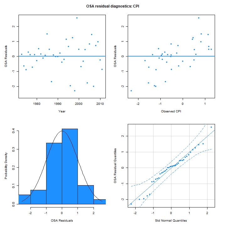
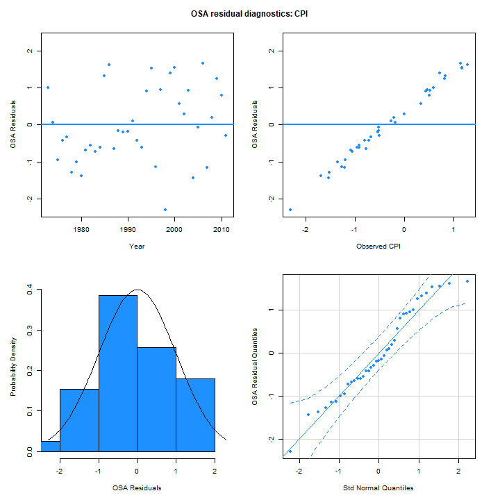
Comparing m4 and m5 demonstrates that the
CPI was best modeled as an AR1 process (m5) instead of a
random walk (m4), since this was the only difference
between the two models and m5 had lower AIC. The
one-step-ahead residuals for the CPI from m5 (right) are
similar in distribution. The linear trend in the OSA residuals with
observed value for m5 is due to the best prediction of the
next observation being near the mean of the process in this case because
the estimated autocorrelation parameter is near 0:
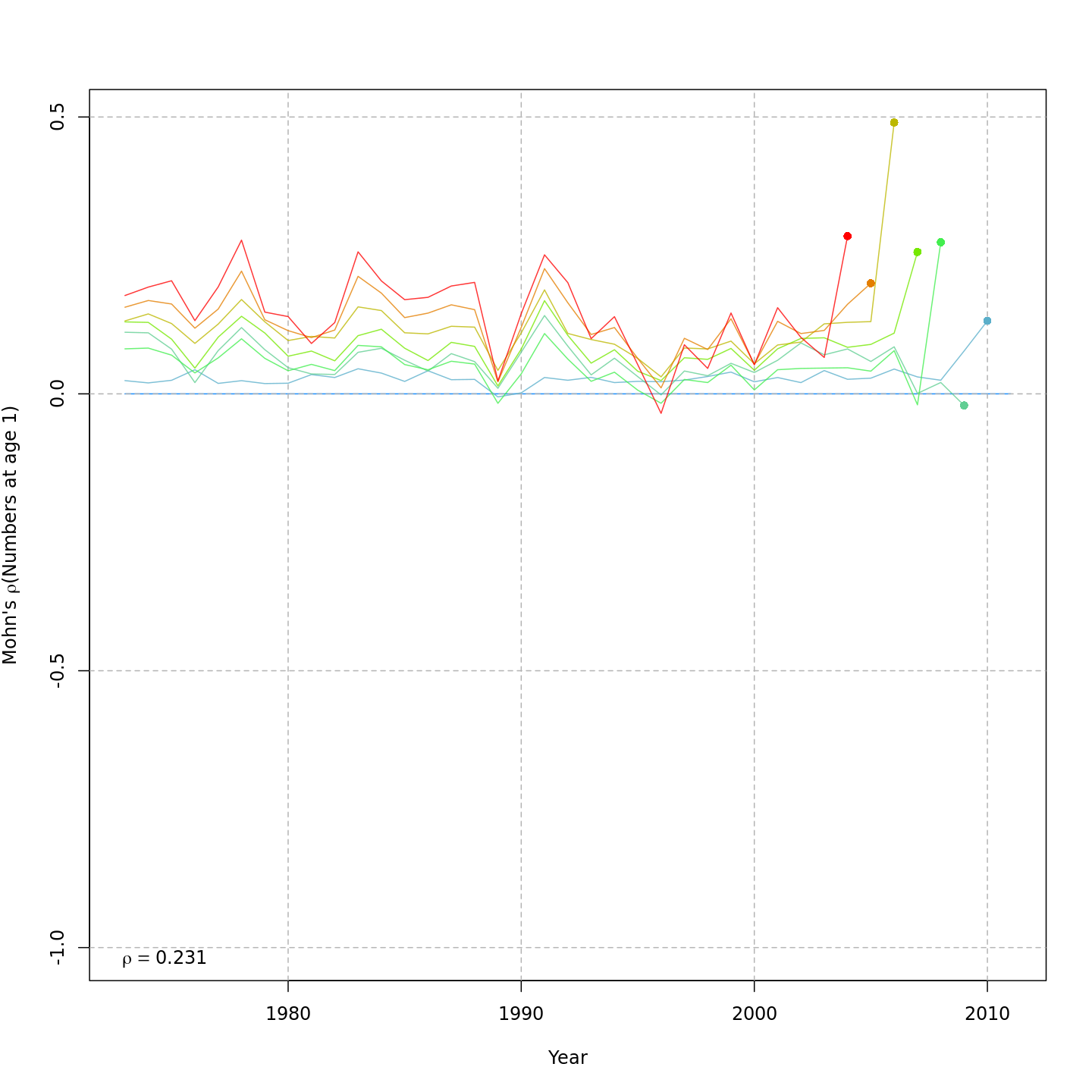
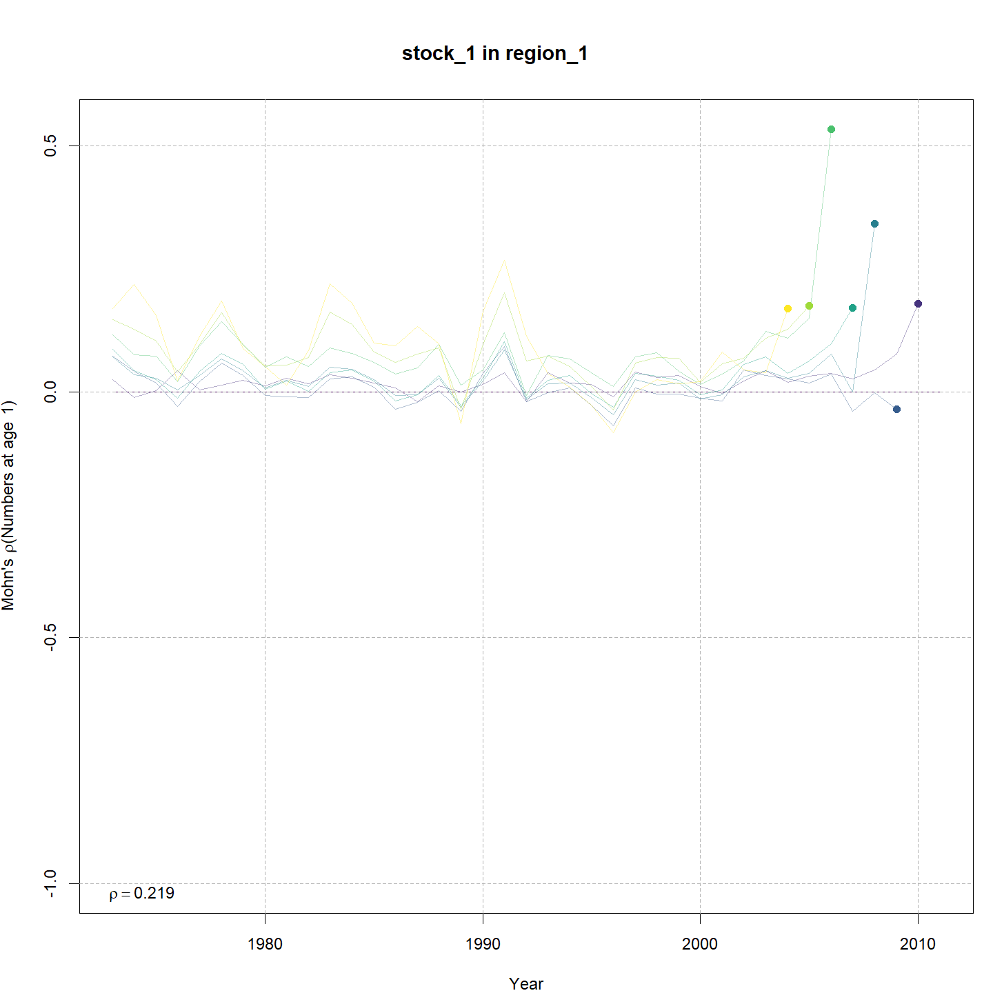
As we saw from the table of results, all the models produced similar
Mohn’s
values for SSB, F, and recruitment. Below are the relative retrospective
peels for the model without any SSB or CPI effects on recruitment
(m1, left) and the best model that included CPI and SSB
effects on recruitment, (m6, right).
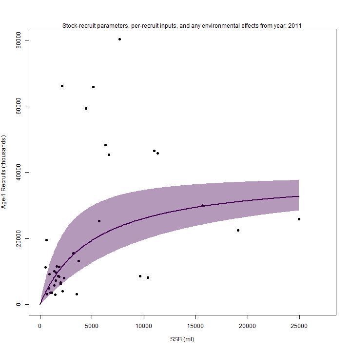
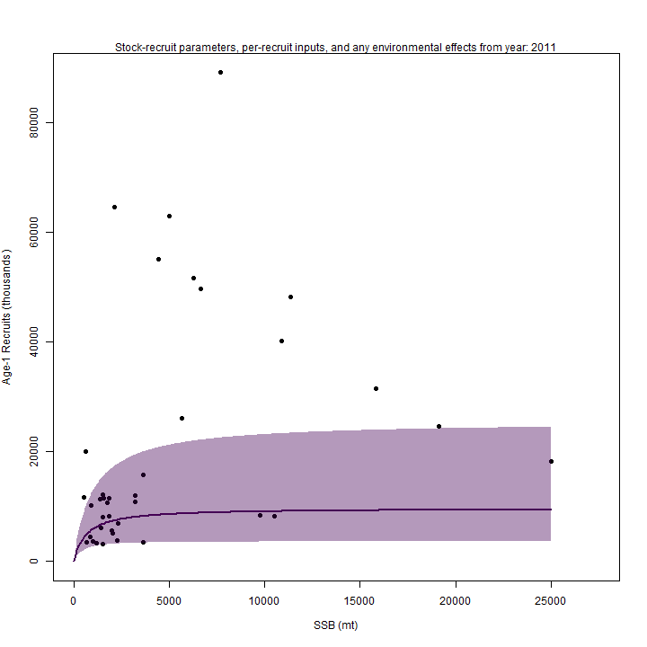
Recruitment
A Beverton-Holt stock-recruitment assumption was preferred over
random recruitment (m3 lower AIC than m1).
Models that included both Bev-Holt and CPI effects on recruitment had
lower AIC than the model with Bev-Holt but without the CPI
(m4 vs. m3). Adding the CPI effect to the
Bev-Holt explains some of the variability around the stock-recruit
curve, which resulted in m4 (right) estimating lower
than m3 (left).
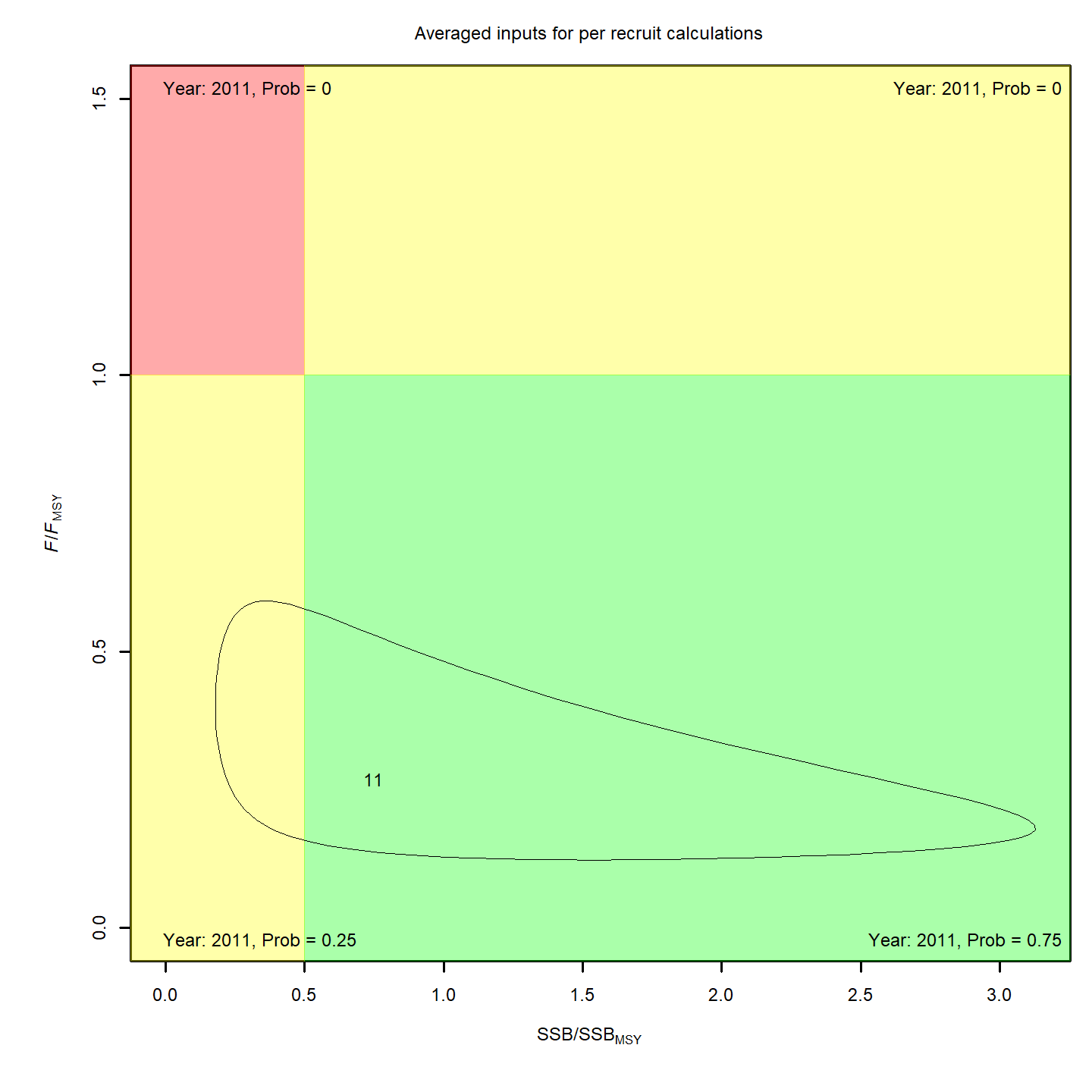
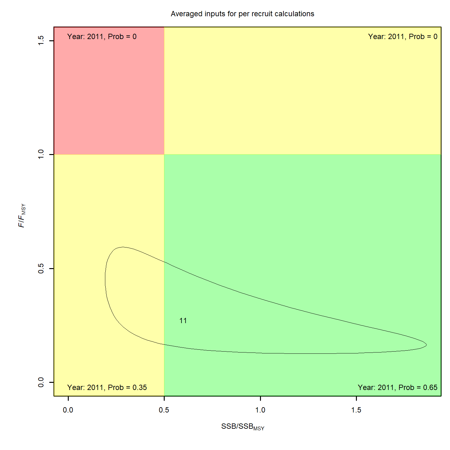
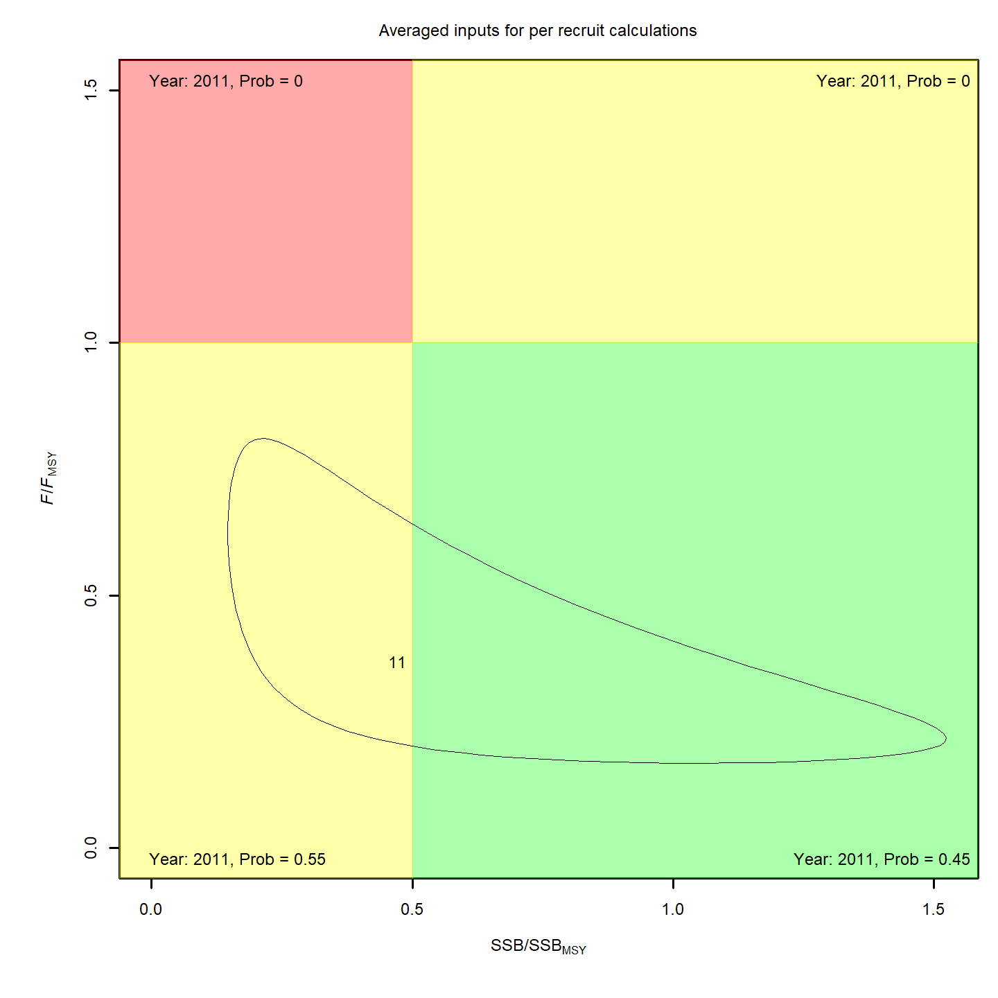
Stock status
Whether or not to include a stock-recruit function and/or the CPI did not have a great influence on estimated stock status using SPR-based reference points. Specifically, the models hardly differed in their estimation of the probability that the stock was overfished, . All models estimated with 100% probability that the stock was not experiencing overfishing in 2011, .
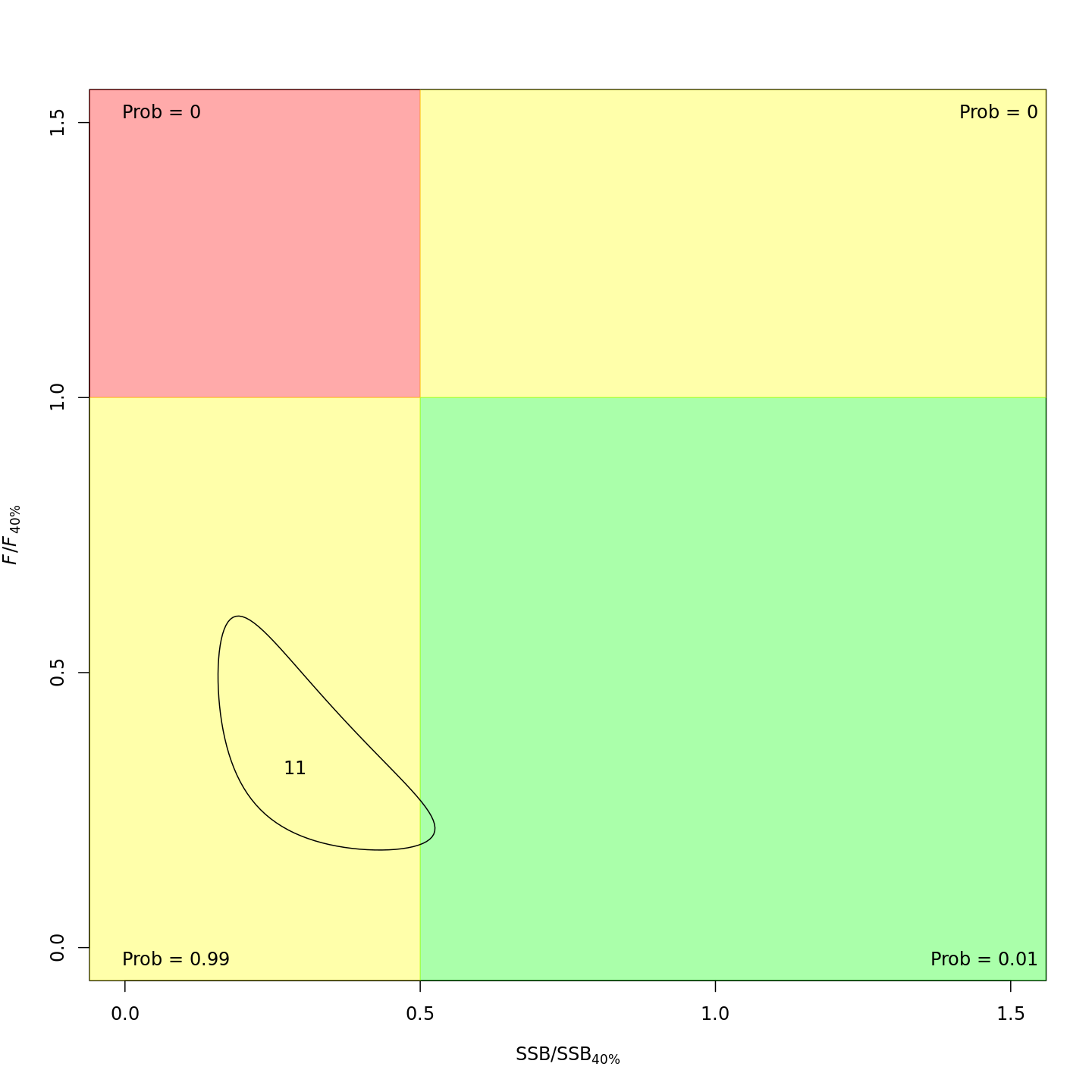


For models with stock recruit functions, status based on MSY-based
reference points is more optimistic: