Ex 4: Selectivity with time- and age-varying random effects
Source:vignettes/ex4_selectivity.Rmd
ex4_selectivity.RmdIn this vignette we walk through an example using the
wham (WHAM = Woods Hole Assessment Model) package to run a
state-space age-structured stock assessment model. WHAM is a
generalization of code written for Miller et al. (2016)
and Xu et
al. (2018), and in this example we apply WHAM to the same stock,
Southern New England / Mid-Atlantic Yellowtail Flounder.
Here we assume you already have wham installed. If not,
see the Introduction.
This is the 4th wham example, which builds off model
m4 from example
1:
full state-space model (numbers-at-age are random effects for all ages,
NAA_re = list(sigma='rec+1',cor='iid'))logistic normal age compositions, treating observations of zero as missing (
age_comp = "logistic-normal-miss0")random-about-mean recruitment (
recruit_model = 2)no environmental covariate (
ecov = NULL)2 indices
fit to 1973-2016 data
In example 4, we demonstrate the time-varying selectivity options in WHAM for both logistic and age-specific selectivity:
none: time-constantiid: parameter- and year-specific (random effect) deviations from mean selectivity parametersar1: as above, but estimate correlation across logistic parametersar1_y: as above, but estimate correlation across years2dar1: as above, but estimate correlation across both years and parameters
Note that each of these options can be applied to any selectivity block (and therefore fleet/catch or index/survey).
1. Load data
Open R and load the wham package:
For a clean, runnable .R script, look at
ex4_selectivity.R in the example_scripts
folder of the wham package install:
wham.dir <- find.package("wham")
file.path(wham.dir, "example_scripts")
You can run this entire example script with:
write.dir <- "choose/where/to/save/output" # otherwise will be saved in working directory
source(file.path(wham.dir, "example_scripts", "ex4_selectivity.R"))
Let’s create a directory for this analysis:
# choose a location to save output, otherwise will be saved in working directory
write.dir <- "choose/where/to/save/output" # need to change
dir.create(write.dir)
setwd(write.dir)
We need the same data files as in example
1. Let’s copy ex1_SNEMAYT.dat to our analysis
directory:
wham.dir <- find.package("wham")
file.copy(from=file.path(wham.dir,"extdata","ex1_SNEMAYT.dat"), to=write.dir, overwrite=FALSE)
Confirm you are in the correct directory and it has the required data files:
list.files()
#>  [1] "age_comp_likelihood_test_values.rds" "BASE_3"
#>  [3] "CPI.csv"                             "ex1_SNEMAYT.dat"
#>  [5] "ex1_test_results.rds"                "ex11_tests.rds"
#>  [7] "ex2_SNEMAYT.dat"                     "ex2_test_results.rds"
#>  [9] "ex4_test_results.rds"                "ex5_summerflounder.dat"
#> [11] "ex5_test_results.rds"                "ex6_test_results.rds"
#> [13] "ex7_SNEMAYT.dat"                     "GSI.csv"
Read the ASAP3 .dat file into R and convert to input list for wham:
asap3 <- read_asap3_dat("ex1_SNEMAYT.dat")2. Specify selectivity model options
We are going to run 9 models that differ only in the selectivity options:
# m1-m5 logistic, m6-m9 age-specific
sel_model <- c(rep("logistic",4), rep("age-specific",5))

# time-varying options for each of 3 blocks (b1 = fleet, b2-3 = indices)
sel_re <- list(c("none","none","none"), # m1-m4 logistic
                c("iid","none","none"),
                c("ar1","none","none"),
                c("2dar1","none","none"),
                c("none","none","none"), # m5-m9 age-specific
                c("iid","none","none"),
                c("ar1","none","none"),
                c("ar1_y","none","none"),
                c("2dar1","none","none"))
n.mods <- length(sel_re)

# summary data frame
df.mods <- data.frame(Model=paste0("m",1:n.mods),
    Selectivity=sel_model, # Selectivity model (same for all blocks)
    Block1_re=sapply(sel_re, function(x) x[[1]])) # Block 1 random effects
rownames(df.mods) <- NULL

df.mods
#>   Model  Selectivity Block1_re
#> 1    m1     logistic      none
#> 2    m2     logistic       iid
#> 3    m3     logistic       ar1
#> 4    m4     logistic     2dar1
#> 5    m5 age-specific      none
#> 6    m6 age-specific       iid
#> 7    m7 age-specific       ar1
#> 8    m8 age-specific     ar1_y
#> 9    m9 age-specific     2dar1
3. Setup and run models
The ASAP data file specifies selectivity options (model, initial
parameter values, which parameters to fix/estimate). WHAM uses these by
default in order to facilitate running ASAP models. To see the currently
specified selectivity options in asap3:
asap3$dat$sel_block_assign # 1 fleet, all years assigned to block 1
#> [[1]]
#>  [1] 1 1 1 1 1 1 1 1 1 1 1 1 1 1 1 1 1 1 1 1 1 1 1 1 1 1 1 1 1 1 1 1 1 1 1 1 1 1
#> [39] 1 1 1 1 1 1
# by default each index gets its own selectivity block (here, blocks 2 and 3)

asap3$dat$sel_block_option # fleet selectivity (1 block), 2 = logistic
#> [1] 2
asap3$dat$index_sel_option # index selectivity (2 blocks), 2 = logistic
#> [1] 2 2

asap3$dat$sel_ini # fleet sel initial values (col1), estimation phase (-1 = fix)
#> [[1]]
#>       [,1] [,2] [,3] [,4]
#>  [1,] 0.10    1    0    1
#>  [2,] 1.00   -1    0    1
#>  [3,] 0.42    1    0    1
#>  [4,] 0.58    1    0    1
#>  [5,] 0.74    1    0    1
#>  [6,] 0.90    1    0    1
#>  [7,] 1.00    2    0    1
#>  [8,] 0.90    3    0    1
#>  [9,] 0.50    1    0    1
#> [10,] 0.60    1    0    1
#> [11,] 4.00    1    0    1
#> [12,] 1.10    1    0    1
asap3$dat$index_sel_ini # index sel initial values (col1), estimation phase (-1 = fix)
#> [[1]]
#>       [,1] [,2] [,3] [,4]
#>  [1,] 0.10    1    0    1
#>  [2,] 0.26    1    0    1
#>  [3,] 1.00   -1    0    1
#>  [4,] 0.58    1    0    1
#>  [5,] 0.74    1    0    1
#>  [6,] 0.90    1    0    1
#>  [7,] 1.50    2    0    1
#>  [8,] 0.90    3    0    1
#>  [9,] 0.75    1    0    1
#> [10,] 0.60    1    0    1
#> [11,] 4.00    1    0    1
#> [12,] 1.10    1    0    1
#>
#> [[2]]
#>       [,1] [,2] [,3] [,4]
#>  [1,] 0.10    1    0    1
#>  [2,] 1.00   -1    0    1
#>  [3,] 0.42    1    0    1
#>  [4,] 0.58    1    0    1
#>  [5,] 0.74    1    0    1
#>  [6,] 0.90    1    0    1
#>  [7,] 1.00    2    0    1
#>  [8,] 0.90    3    0    1
#>  [9,] 0.50    1    0    1
#> [10,] 0.60    1    0    1
#> [11,] 4.00    1    0    1
#> [12,] 1.10    1    0    1
When we specify the WHAM model with
prepare_wham_input(), we can overwrite the selectivity
options from the ASAP data file with the optional list argument
selectivity. The selectivity model is chosen via
selectivity$model:
| Model | selectivity$model |
No. Parameters |
|---|---|---|
| Age-specific | "age-specific" |
n_ages |
| Logistic (increasing) | "logistic" |
2 |
| Double logistic (dome) | "double-logistic" |
4 |
| Logistic (decreasing) | "decreasing-logistic" |
2 |
Regardless of the selectivity model used, we incorporate time-varying selectivity by estimating a mean for each selectivity parameter, \(\mu^{s}_a\), and (random effect) deviations from the mean, \(\delta_{a,y}\). We then estimate the selectivity parameters, \(s_{a,y}\), on the logit-scale with (possibly) lower and upper limits: \[s_{a,y} = \mathrm{lower} + \frac{\mathrm{upper} - \mathrm{lower}}{1 + e^{-(\mu^{s}_a + \delta_{a,y})}}\]
The deviations, \(\boldsymbol{\delta}\), follow a 2-dimensional AR(1) process defined by the parameters \(\sigma^2_s\), \(\rho_a\), and \(\rho_y\): \[\boldsymbol{\delta} \sim \mathrm{MVN}(0,\Sigma)\] \[\Sigma = \sigma^2_s(\mathrm{R}_a \otimes \mathrm{R}_y)\] \[R_{a,a^*} = \rho_a^{\vert a - a^* \vert}\] \[R_{y,y^*} = \rho_y^{\vert y - y^* \vert}\]
Mean selectivity parameters can be initialized at different values
from the ASAP file with selectivity$initial_pars.
Parameters can be fixed at their initial values by specifying
selectivity$fix_pars. Finally, we specify any time-varying
(random effects) on selectivity parameters
(selectivity$re):
selectivity$re |
Deviations from mean | Estimated parameters |
|---|---|---|
"none" |
time-constant (no deviation) | |
"iid" |
independent, identically-distributed | \(\sigma^2\) |
"ar1" |
autoregressive-1 (correlated across ages/parameters) | \(\sigma^2\), \(\rho_a\) |
"ar1_y" |
autoregressive-1 (correlated across years) | \(\sigma^2\), \(\rho_y\) |
"2dar1" |
2D AR1 (correlated across both years and ages/parameters) | \(\sigma^2\), \(\rho_a\), \(\rho_y\) |
Now we can run the above models in a loop:
for(m in 1:n.mods){
    if(sel_model[m] == "logistic"){ # logistic selectivity
        # overwrite initial parameter values in ASAP data file (ex1_SNEMAYT.dat)
        input <- prepare_wham_input(asap3, model_name=paste(paste0("Model ",m), sel_model[m], paste(sel_re[[m]], collapse="-"), sep=": "), recruit_model=2,
                    selectivity=list(model=rep("logistic",3), re=sel_re[[m]], initial_pars=list(c(2,0.3),c(2,0.3),c(2,0.3))),
                    NAA_re = list(sigma='rec+1',cor='iid'),
                    age_comp = "logistic-normal-miss0") # logistic normal, treat 0 obs as missing
    } else { # age-specific selectivity
        # # you can try not fixing any ages first
        # input <- prepare_wham_input(asap3, model_name=paste(paste0("Model ",m), sel_model[m], paste(sel_re[[m]], collapse="-"), sep=": "), recruit_model=2,
        #           selectivity=list(model=rep("age-specific",3), re=sel_re[[m]],
        #               initial_pars=list(rep(0.5,6), rep(0.5,6), rep(0.5,6))),
        #           NAA_re = list(sigma='rec+1',cor='iid'),
        #           age_comp = "logistic-normal-miss0") # logistic normal, treat 0 obs as missing

        # often need to fix selectivity = 1 for at least one age per age-specific block: ages 4-6 / 4 / 3-6
        input <- prepare_wham_input(asap3, model_name=paste(paste0("Model ",m), sel_model[m], paste(sel_re[[m]], collapse="-"), sep=": "), recruit_model=2,
                    selectivity=list(model=rep("age-specific",3), re=sel_re[[m]],
                        initial_pars=list(c(0.1,0.5,0.5,1,1,1),c(0.5,0.5,0.5,1,0.5,0.5),c(0.5,0.5,1,1,1,1)),
                        fix_pars=list(4:6,4,3:6)),
                    NAA_re = list(sigma='rec+1',cor='iid'),
                    age_comp = "logistic-normal-miss0") # logistic normal, treat 0 obs as missing
    }

    # fit model
    mod <- fit_wham(input, do.check=T, do.osa=F, do.proj=F, do.retro=F)
    saveRDS(mod, file=paste0("m",m,".rds"))
}
4. Model convergence and comparison
Collect all models into a list:
Check which models converged.
vign4_conv <- lapply(mods, function(x) capture.output(check_convergence(x)))
for(m in 1:n.mods) cat(paste0("Model ",m,":"), vign4_conv[[m]], "", sep='\n')
#> Model 1:
#> stats:nlminb thinks the model has converged: mod$opt$convergence == 0
#> Maximum gradient component: 2.04e-01
#> Max gradient parameter: logit_selpars
#> TMB:sdreport() was performed successfully for this model
#>
#> Model 2:
#> stats:nlminb thinks the model has converged: mod$opt$convergence == 0
#> Maximum gradient component: 2.27e-01
#> Max gradient parameter: logit_selpars
#> TMB:sdreport() was performed successfully for this model
#>
#> Model 3:
#> stats:nlminb thinks the model has converged: mod$opt$convergence == 0
#> Maximum gradient component: 2.04e-01
#> Max gradient parameter: logit_selpars
#> TMB:sdreport() was performed successfully for this model
#>
#> Model 4:
#> stats:nlminb thinks the model has converged: mod$opt$convergence == 0
#> Maximum gradient component: 2.26e-01
#> Max gradient parameter: logit_selpars
#> TMB:sdreport() was performed successfully for this model
#>
#> Model 5:
#> stats:nlminb thinks the model has converged: mod$opt$convergence == 0
#> Maximum gradient component: 2.10e-01
#> Max gradient parameter: F_devs
#> TMB:sdreport() was performed successfully for this model
#>
#> Model 6:
#> stats:nlminb thinks the model has converged: mod$opt$convergence == 0
#> Maximum gradient component: 2.10e-01
#> Max gradient parameter: F_devs
#> TMB:sdreport() was performed successfully for this model
#>
#> Model 7:
#> stats:nlminb thinks the model has converged: mod$opt$convergence == 0
#> Maximum gradient component: 2.10e-01
#> Max gradient parameter: F_devs
#> TMB:sdreport() was performed successfully for this model
#>
#> Model 8:
#> stats:nlminb thinks the model has converged: mod$opt$convergence == 0
#> Maximum gradient component: 2.25e-01
#> Max gradient parameter: F_devs
#> TMB:sdreport() was performed successfully for this model
#>
#> Model 9:
#> stats:nlminb thinks the model has converged: mod$opt$convergence == 0
#> Maximum gradient component: 2.27e-01
#> Max gradient parameter: F_devs
#> TMB:sdreport() was performed successfully for this modelPlot output for models that converged (in a subfolder for each model):
# Is Hessian positive definite?
ok_sdrep = sapply(mods, function(x) if(x$na_sdrep==FALSE & !is.na(x$na_sdrep)) 1 else 0)
pdHess <- as.logical(ok_sdrep)
# did stats::nlminb converge?
conv <- sapply(mods, function(x) x$opt$convergence == 0) # 0 means opt converged
conv_mods <- (1:n.mods)[pdHess]
for(m in conv_mods){
    plot_wham_output(mod=mods[[m]], out.type='html', dir.main=file.path(write.dir,paste0("m",m)))
}
Compare the models using AIC:
df.aic <- as.data.frame(compare_wham_models(mods, table.opts=list(sort=FALSE, calc.rho=FALSE))$tab)
df.aic[!pdHess,] = NA
minAIC <- min(df.aic$AIC, na.rm=T)
df.aic$dAIC <- round(df.aic$AIC - minAIC,1)
df.mods <- cbind(data.frame(Model=paste0("m",1:n.mods), Selectivity=sel_model,
                            "Block1_re"=sapply(sel_re, function(x) x[[1]]),
                            "opt_converged"= ifelse(conv, "Yes", "No"),
                            "pd_hessian"= ifelse(pdHess, "Yes", "No"),
                            "NLL"=sapply(mods, function(x) round(x$opt$objective,3)),
                            "Runtime"=sapply(mods, function(x) x$runtime)), df.aic)
rownames(df.mods) <- NULL
df.mods
#> Model Selectivity Block1_re opt_converged pd_hessian NLL Runtime dAIC
#> 1 m1 logistic none Yes Yes -795.146 0.23 47.6
#> 2 m2 logistic iid Yes Yes -814.967 0.31 10.0
#> 3 m3 logistic ar1 Yes Yes -795.146 0.34 51.6
#> 4 m4 logistic 2dar1 Yes Yes -821.965 0.36 0.0
#> 5 m5 age-specific none Yes Yes -800.055 0.23 45.8
#> 6 m6 age-specific iid Yes Yes -800.055 0.84 47.8
#> 7 m7 age-specific ar1 Yes Yes -800.055 0.84 49.8
#> 8 m8 age-specific ar1_y Yes Yes -822.528 0.31 4.8
#> 9 m9 age-specific 2dar1 Yes Yes -823.888 1.23 4.1
#> AIC
#> 1 -1462.3
#> 2 -1499.9
#> 3 -1458.3
#> 4 -1509.9
#> 5 -1464.1
#> 6 -1462.1
#> 7 -1460.1
#> 8 -1505.1
#> 9 -1505.8Prepare to plot selectivity-at-age for block 1 (fleet).
library(tidyverse)
library(viridis)

sel_mod <- factor(c("Age-specific","Logistic")[sapply(mods, function(x) x$env$data$selblock_models[1])], levels=c("Logistic","Age-specific"))
sel_cor <- factor(c("None","IID","AR1","AR1_y","2D AR1")[sapply(mods, function(x) x$env$data$selblock_models_re[1])], levels=c("None","IID","AR1","AR1_y","2D AR1"))
df.selAA <- data.frame(matrix(NA, nrow=0, ncol=11))
colnames(df.selAA) <- c(paste0("Age_",1:6),"Year","Model","conv","sel_mod","sel_cor")
for(m in 1:n.mods){
    df <- as.data.frame(selAA[[m]])
    df$Year <- input$years
    colnames(df) <- c(paste0("Age_",1:6),"Year")
    df$Model <- m
    df$conv <- ifelse(df.mods$pd_hessian[m]=="Yes",1,0)
    df$sel_mod = sel_mod[m]
    df$sel_cor = sel_cor[m]
    df.selAA <- rbind(df.selAA, df)
}
df <- df.selAA %>% pivot_longer(-c(Year,Model,conv,sel_mod,sel_cor),
                names_to = "Age",
                names_prefix = "Age_",
                names_transform = list(Age = as.integer),
                values_to = "Selectivity")
df$Age <- as.integer(df$Age)
df$sel_mod <- factor(df$sel_mod, levels=c("Logistic","Age-specific"))
df$sel_cor <- factor(df$sel_cor, levels=c("None","IID","AR1","AR1_y","2D AR1"))
df$conv = factor(df$conv)
Now plot selectivity-at-age for block 1 (fleet) in all models.
print(ggplot(df, aes(x=Year, y=Age)) +
    geom_tile(aes(fill=Selectivity)) +
    geom_label(aes(x=Year, y=Age, label=lab), size=5, alpha=1, #fontface = "bold",
      data=data.frame(Year=1975.5, Age=5.8, lab=paste0("m",1:length(mods)), sel_mod=sel_mod, sel_cor=sel_cor)) +
    facet_grid(rows=vars(sel_cor), cols=vars(sel_mod)) +
    scale_fill_viridis() +
    theme_bw() +
    scale_x_continuous(expand=c(0,0)) +
    scale_y_continuous(expand=c(0,0)))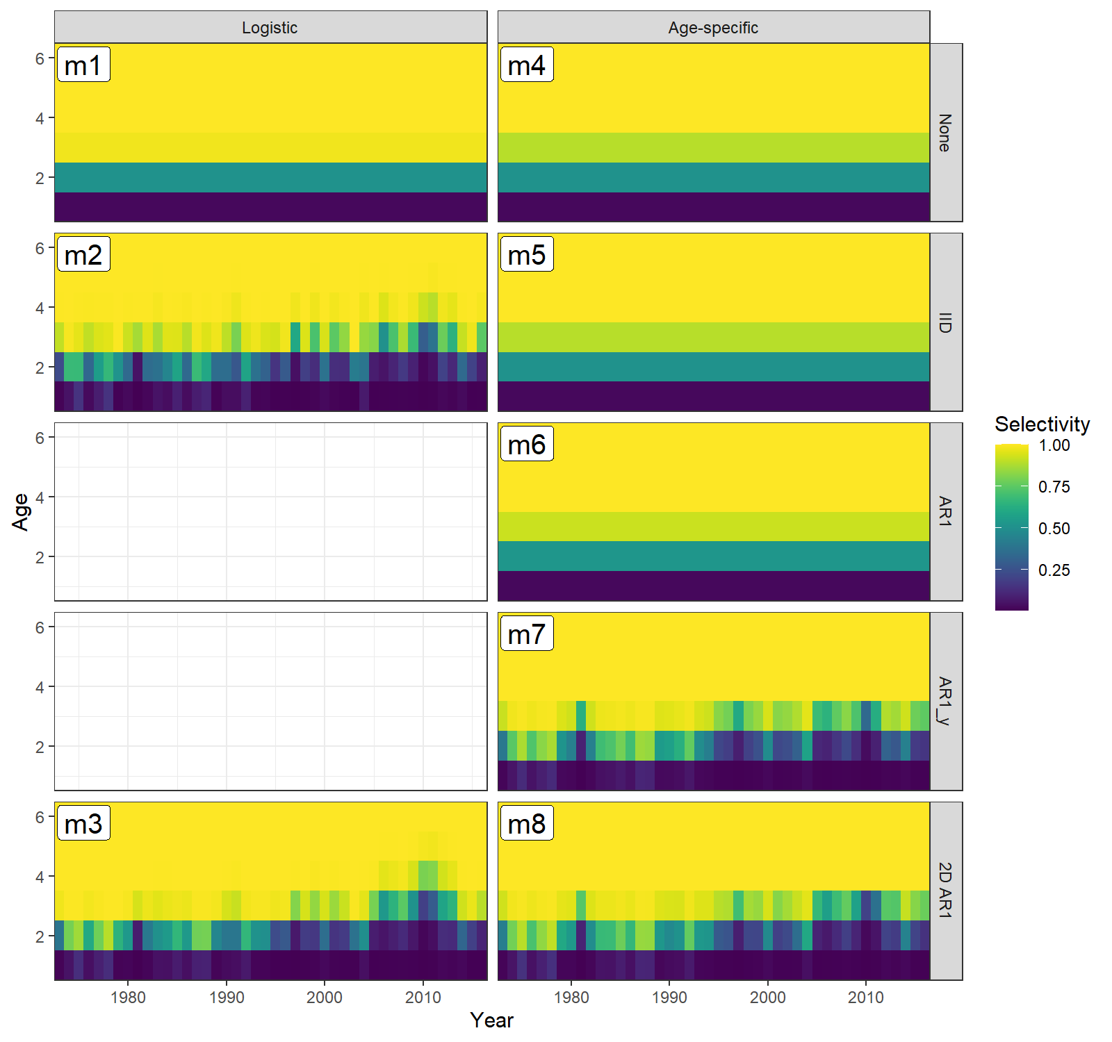
A note on convergence
When fitting age-specific selectivity, oftentimes some of the (mean, \(\mu^{s}_a\)) selectivity parameters need to be fixed for the model to converge. The specifications used here follow this procedure:
- Fit the model without fixing any selectivity parameters.
- If the model fails to converge or the hessian is not invertible
(i.e. not positive definite), look for mean selectivity parameters that
are very close to 0 or 1 (> 5 or < -5 on the logit scale) and/or
have
NaNestimates of their standard error:
mod$rep$logit_selpars # mean sel pars
mod$rep$sel_repars # if time-varying selectivity turned on
mod$rep$selAA # selectivity-at-age by block
mod$sdrep # look for sel pars with NaN standard errors- Re-run the model fixing the worst selectivity-at-age parameter for each block at 0 or 1 as appropriate. In the above age-specific models, we first initialized and fixed ages 4, 4, and 2 for blocks 1-3, respectively. The logit scale selectivity for age 5 and ages 3-4 for blocks 1 and 3 remained around 20, indicating that they too should be fixed at 1. Sometimes just initializing the worst parameter is enough, without fixing it.
        # fix selectivity at 1 for ages 4-5 / 4 / 2-4 in blocks 1-3
        input <- prepare_wham_input(asap3, model_name=paste(paste0("Model ",m), sel_model[m], paste(sel_re[[m]], collapse="-"), sep=": "), recruit_model=2,
                    selectivity=list(model=rep("age-specific",3), re=sel_re[[m]],
                        initial_pars=list(c(0.1,0.5,0.5,1,1,0.5),c(0.5,0.5,0.5,1,0.5,0.5),c(0.5,1,1,1,0.5,0.5)),
                        fix_pars=list(4:5,4,2:4)),
NAA_re = list(sigma='rec+1',cor='iid'))- The goal is to find a set of selectivity parameter initial/fixed values that allow all nested models to converge. Fixing parameters should not affect the NLL much, and any model that is a superset of another should not have a greater NLL (indicates not converged to global minimum). The following commands may be helpful: