This is the 8th WHAM example. We assume you already have
wham installed and are relatively familiar with the
package. If not, read the Introduction and Tutorial.
In this vignette we show how to read in ASAP3 model results and
compare to WHAM models, using the compare_wham_models()
function. We use the 2019
Georges Bank haddock stock assessment, which is an update to the VPA
benchmark (NEFSC
2008). Thanks to Liz Brooks for sharing the ASAP3 data file and
model output in preparation for the 2021 research track assessment–these
files and results are very preliminary.
# devtools::install_github("timjmiller/wham", dependencies=TRUE)
library(tidyverse)
#> Warning: package 'ggplot2' was built under R version 4.2.3
#> Warning: package 'tibble' was built under R version 4.2.3
#> Warning: package 'tidyr' was built under R version 4.2.3
#> Warning: package 'purrr' was built under R version 4.2.3
#> Warning: package 'dplyr' was built under R version 4.2.3
#> Warning: package 'stringr' was built under R version 4.2.3
library(wham)
Create a directory for this analysis:
# choose a location to save output, otherwise will be saved in working directory
write.dir <- "choose/where/to/save/output"
dir.create(write.dir)
setwd(write.dir)
The Georges Bank haddock ASAP data file is distributed in
wham. Read in the ASAP file, BASE_3.DAT.
wham.dir <- find.package("wham")
asap.dir <- file.path(wham.dir,"extdata","BASE_3")
asap3 <- read_asap3_dat(file.path(asap.dir,"BASE_3.DAT"))
Define three basic WHAM models with different numbers-at-age random effects:
-
m1: similar to ASAP, where recruitment deviations in each year are estimated as fixed effect parameters. -
m2: recruitment as random effects, estimating \(\sigma^2_R\). -
m3: all numbers-at-age are random effects, i.e. the full state-space model.
df.mods <- data.frame(naa_sig=c('none','rec','rec+1'), naa_cor=c('none','iid','iid'))
n.mods <- dim(df.mods)[1]
df.mods$Model <- paste0("m",1:n.mods)
df.mods <- df.mods %>% select(Model, everything()) # moves Model to first col

# look at model table
df.mods
#>   Model naa_sig naa_cor
#> 1    m1    none    none
#> 2    m2     rec     iid
#> 3    m3   rec+1     iid
Run the WHAM models
All models use the same options for expected recruitment (random
about mean, no stock-recruit function) and selectivity as specified in
BASE_3.DAT.
for(m in 1:n.mods){
  NAA_list <- list(cor=df.mods[m,"naa_cor"], sigma=df.mods[m,"naa_sig"])
  if(NAA_list$sigma == 'none') NAA_list = NULL

  input <- prepare_wham_input(asap3, recruit_model = 2,
                              model_name = df.mods$Model[m],
                              NAA_re = NAA_list)

  mod <- fit_wham(input, do.osa=F)
  saveRDS(mod, file=file.path(write.dir, paste0(df.mods$Model[m],".rds")))
}
Look at convergence and diagnostics
mod.list <- file.path(write.dir,paste0("m",1:n.mods,".rds"))
mods <- lapply(mod.list, readRDS)
ok_sdrep = sapply(mods, function(x) if(x$na_sdrep==FALSE & !is.na(x$na_sdrep)) 1 else 0)
df.mods$conv <- sapply(mods, function(x) x$opt$convergence == 0) # 0 means opt converged
df.mods$pdHess <- as.logical(ok_sdrep)
conv_mods <- (1:n.mods)[df.mods$pdHess]
for(m in conv_mods){
  plot_wham_output(mod=mods[[m]], out.type='pdf', dir.main=file.path(write.dir,paste0("m",m)))
}
Get output from ASAP model run using read_asap3_fit().
Then combine the ASAP model and 3 WHAM models into a named list,
mods.
Comparison plots
Now we can use compare_wham_models() to plot key output
from all 4 models together for comparison.
res <- compare_wham_models(mods, fdir=write.dir, plot.opts=list(kobe.prob=FALSE))
saveRDS(res, file=file.path(write.dir,"res.rds"))
There are many options, see ?compare_wham_models. To
only get the AIC and retro table, not plots (note that ASAP models
cannot be included here).
res <- compare_wham_models(mods, fdir=write.dir, do.plot=F)
round(res$tab,2)
#> dAIC AIC rho_R rho_SSB rho_Fbar
#> WHAM-m1 0.0 5775.7 0.82 0.28 -0.23
#> WHAM-m3 123.3 5899.0 0.31 0.16 -0.16
#> WHAM-m2 355.6 6131.3 0.73 0.27 -0.23Only get the plots, not the table
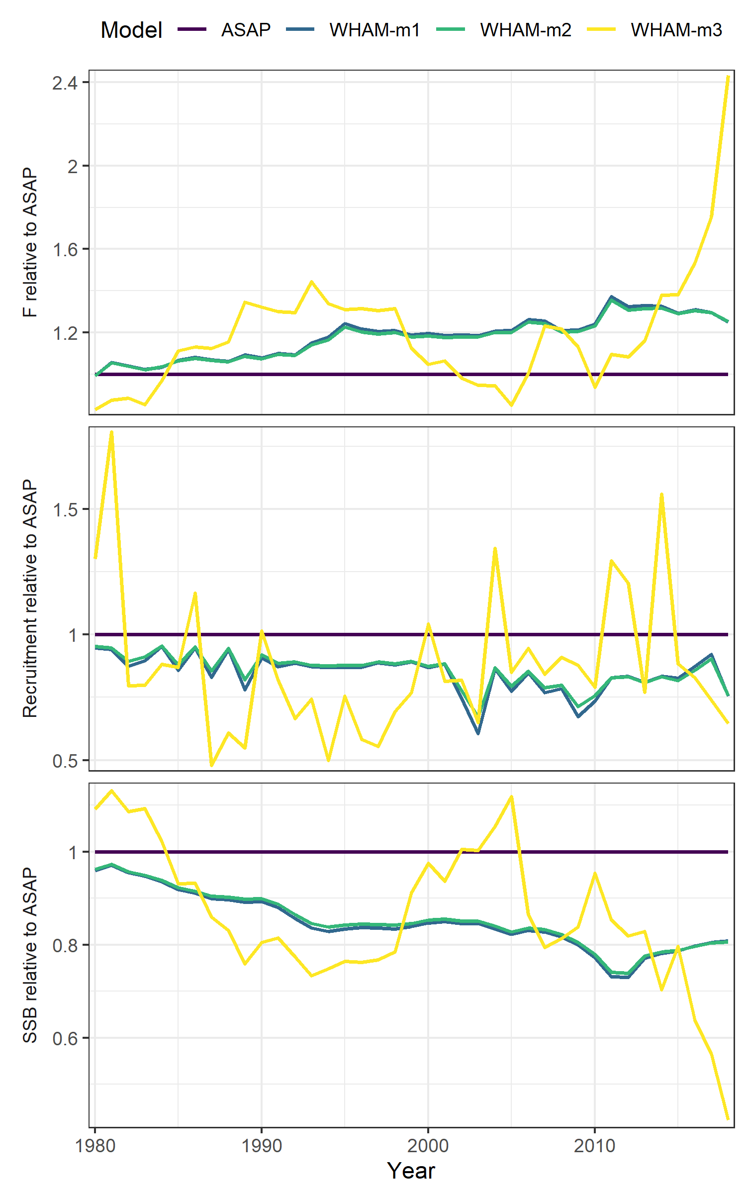
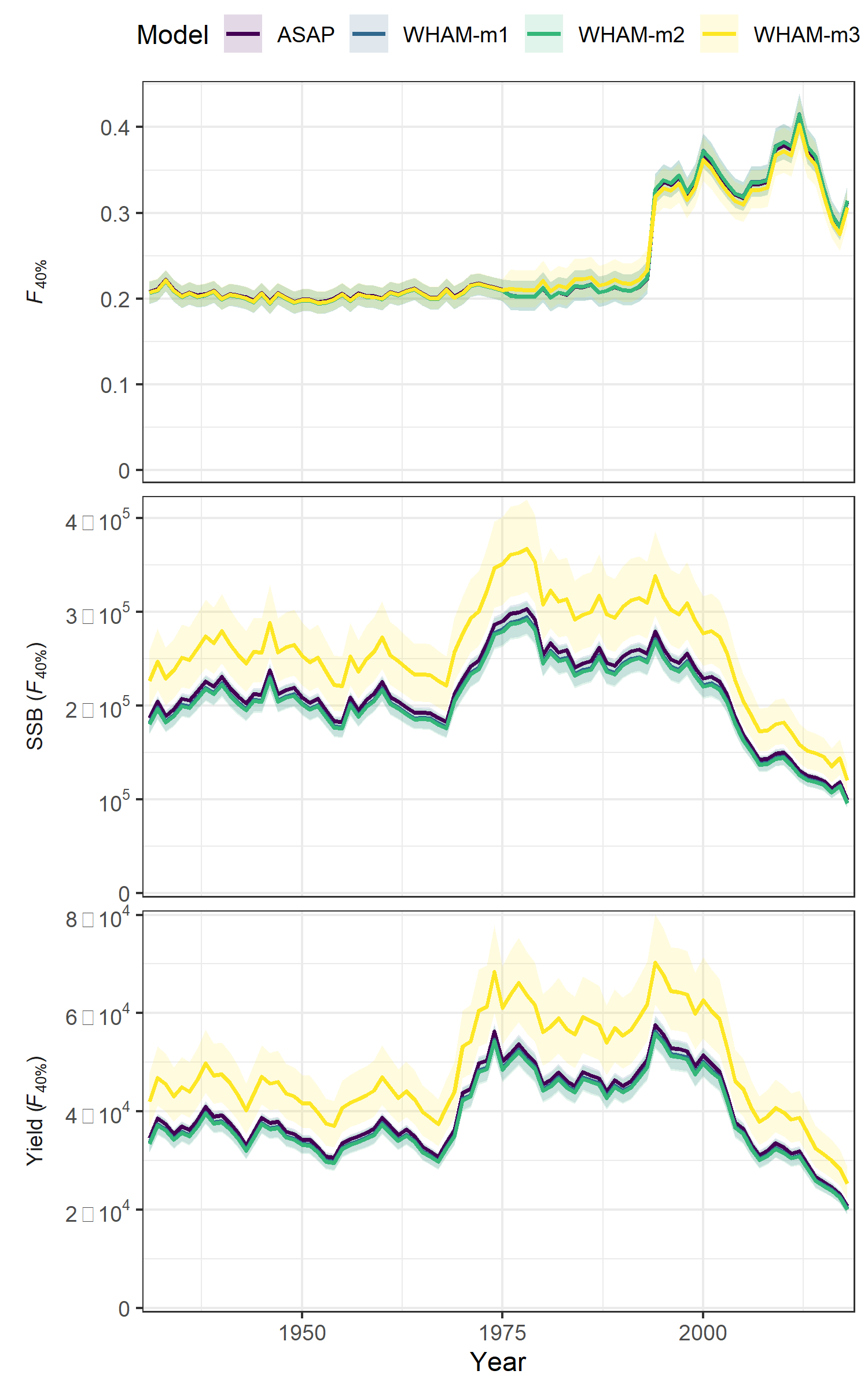
res <- compare_wham_models(mods, fdir=write.dir, do.table=F)Plot 1: 3-panel of SSB (spawning stock biomass), F (fully-selected fishing mortality), and Recruitment
Modifying comparison plots
Many modifications can be made using built-in options, see
$plot.opts in compare_wham_models().
Plots are saved as png by default, can be pdf
res <- compare_wham_models(mods, fdir=write.dir, plot.opts=list(out.type='pdf'))$which lets you choose which of the plots to make
$years lets you only plot a subset of model years
# which = 9 (only plot relative status)
# years = 1980-2018
compare_wham_models(mods, do.table=F, plot.opts=list(years=1980:2018, which=9))
ggsave(file.path(write.dir,"which9_zoom.png"), device='png', width=6.5, height=5.5, units='in')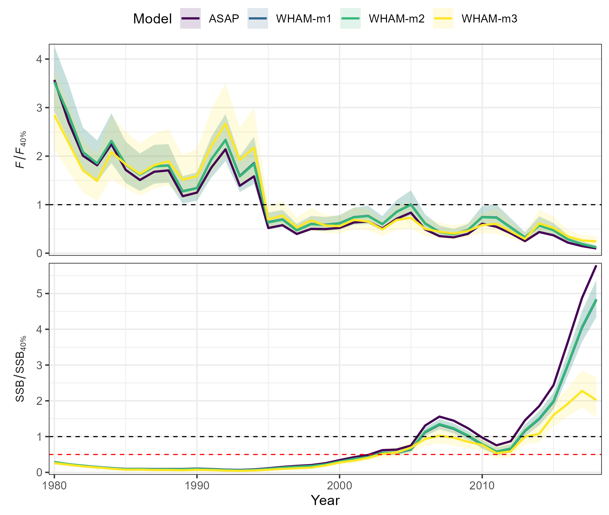
$ci can turn off the confidence interval shading for all
or some models
# which = 1 (SSB, F, recruitment)
# ci = FALSE (remove confidence intervals for all models, can also choose a subset)
compare_wham_models(mods, fdir=write.dir, do.table=F, plot.opts=list(ci=FALSE, which=1))
ggsave(file.path(write.dir,"which1_noCI.png"), device='png', width=6.5, height=5.5, units='in')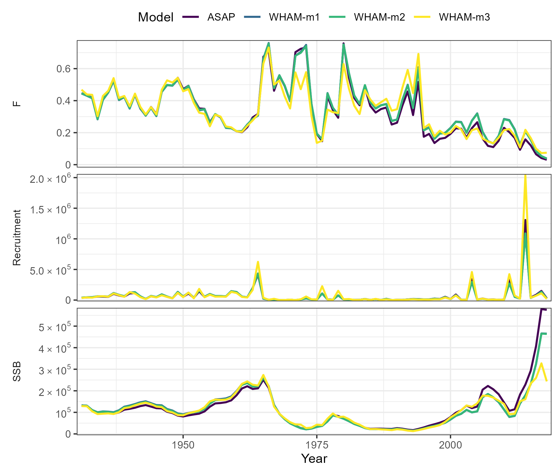
$relative.to lets you plot differences between the
models relative to a base model (here, ASAP)
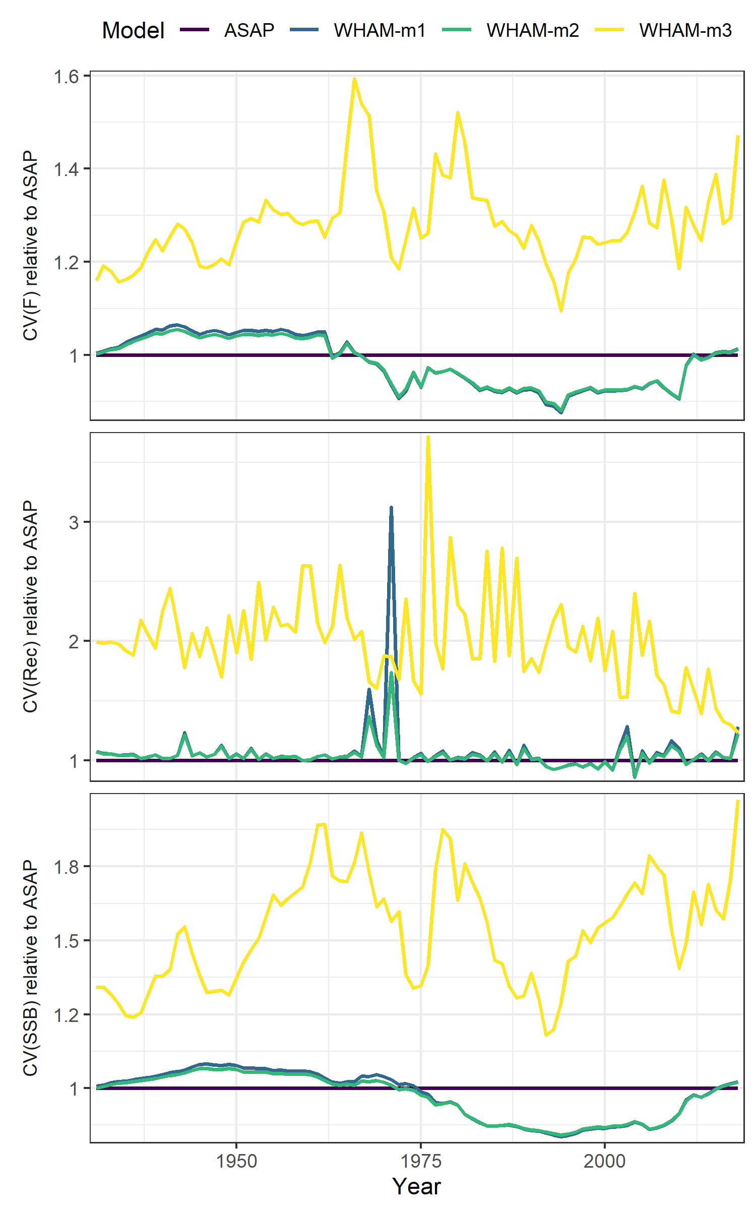
# which = 2 (CV of SSB, F, recruitment)
# relative to ASAP
compare_wham_models(mods, fdir=write.dir, do.table=F, plot.opts=list(ci=FALSE, relative.to="ASAP", which=2))
ggsave(file.path(write.dir,"which2_relative.png"), device='png', width=6.5, height=5.5, units='in')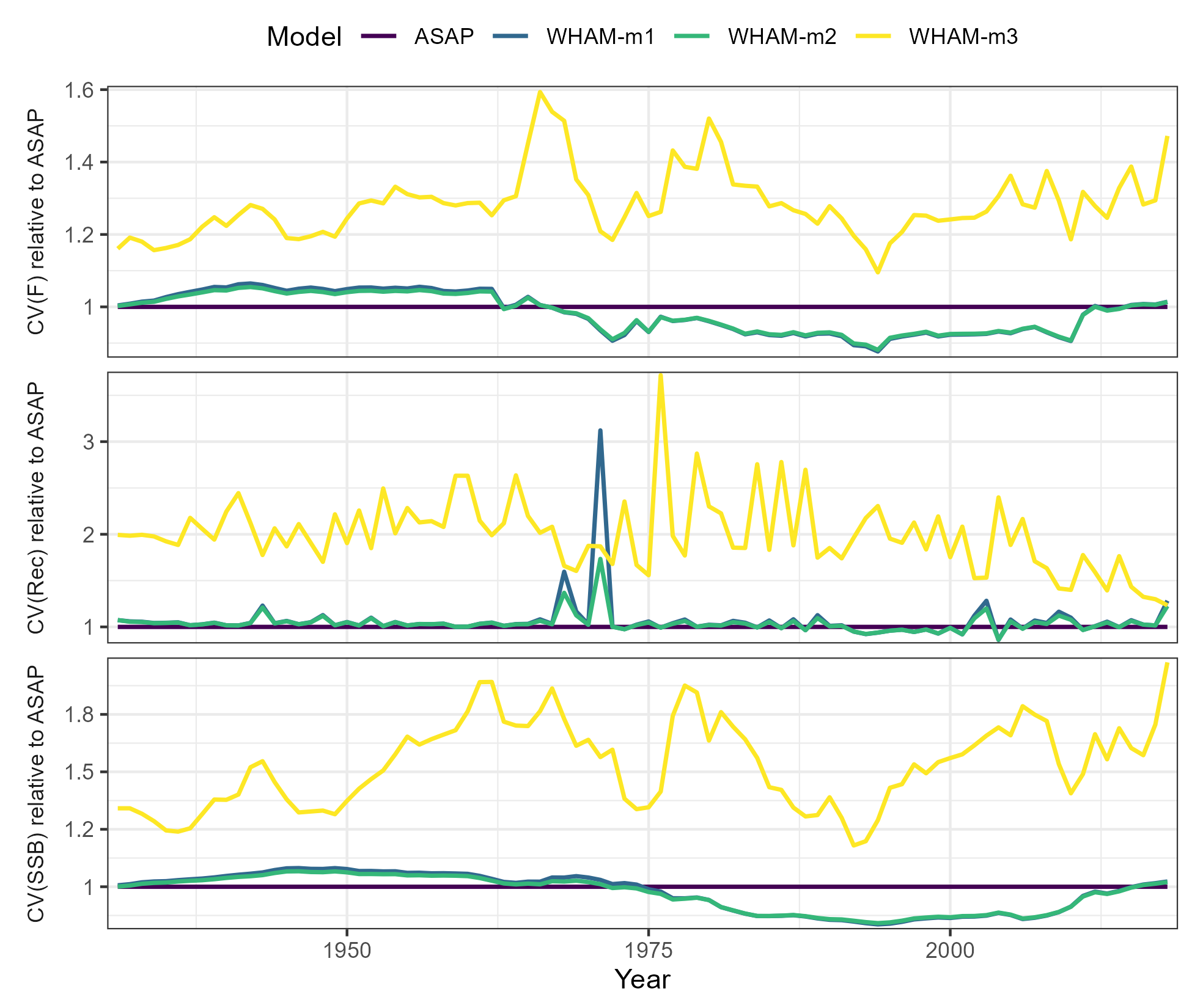
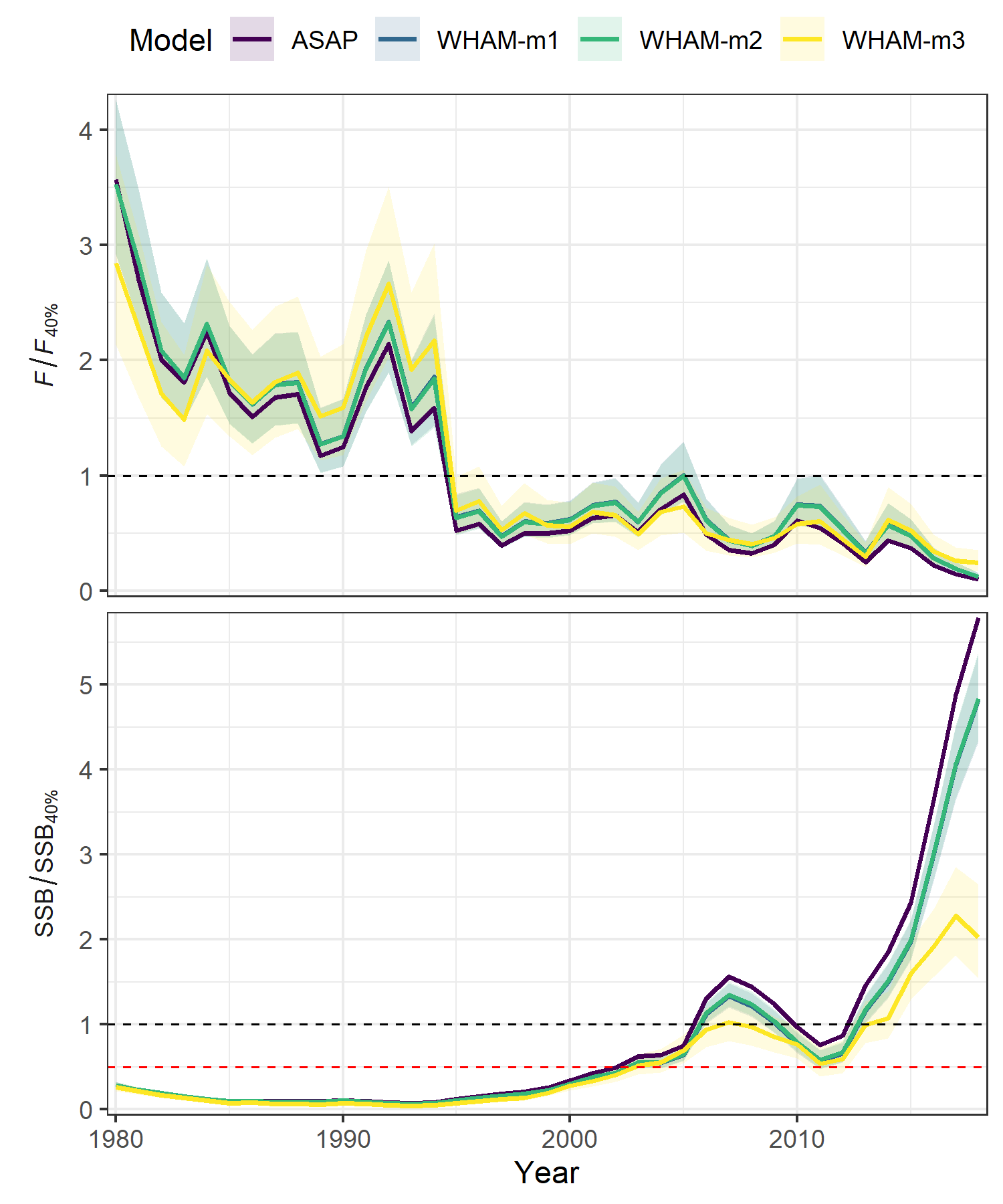
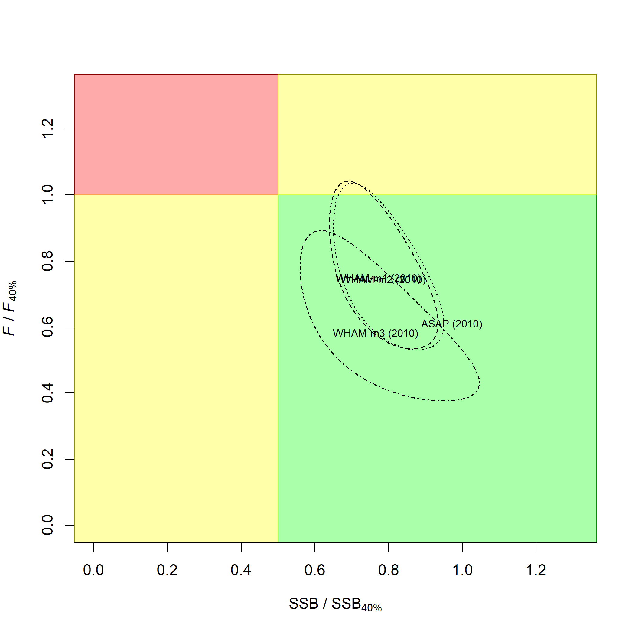
$kobe.yr is used to specify the year in the Kobe
relative status plot $kobe.prob = F will turn off the
probabilities printed in each quadrant for each model (can be crowded
with many models)
# which = 10 (kobe plot)
# kobe.yr = 2010 (instead of terminal year, 2018)
# kobe.prob = F (don't print probabilities)
compare_wham_models(mods, fdir=write.dir, do.table=F, plot.opts=list(which=10, kobe.yr=2010, kobe.prob=F))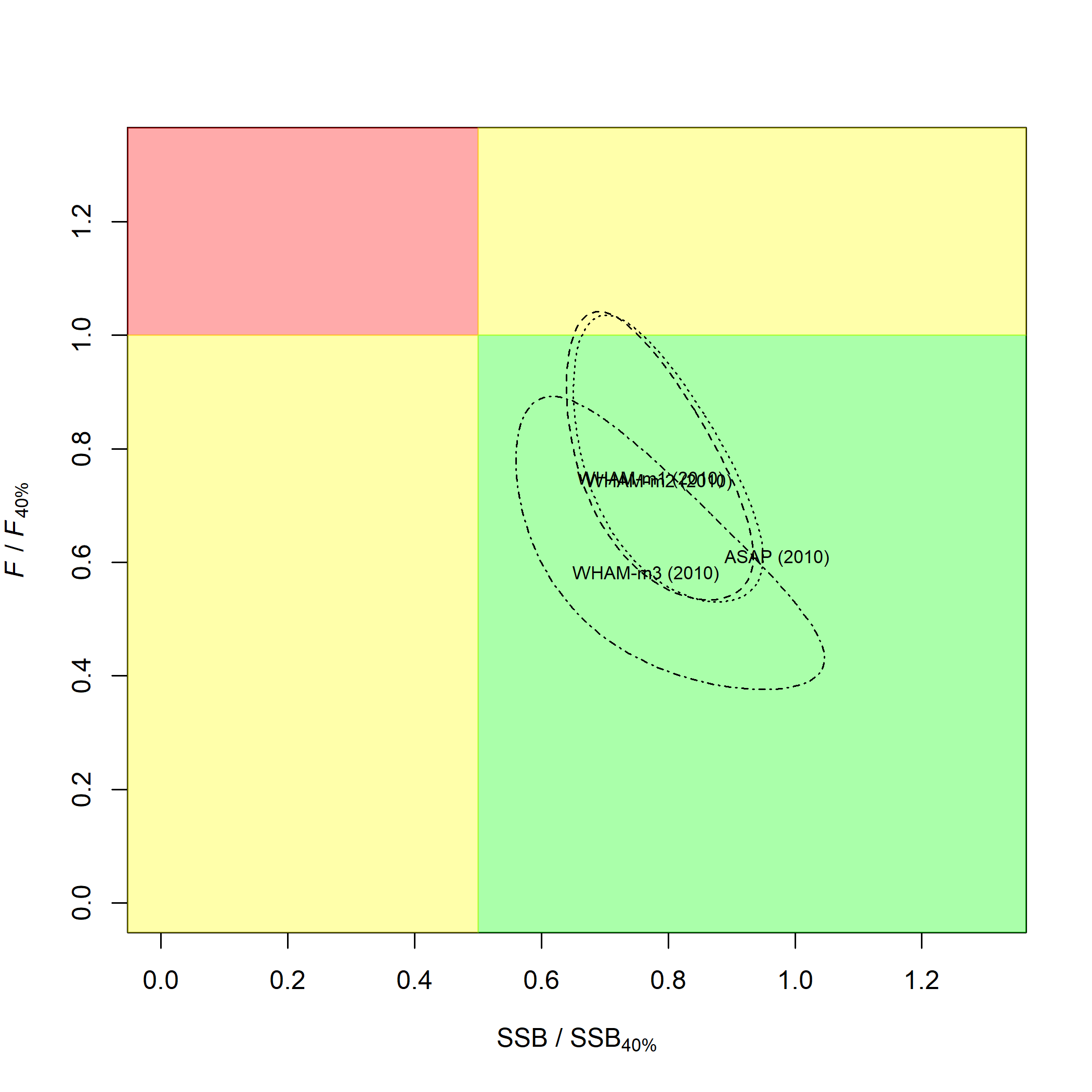
The plots made with ggplot2 (all except Kobe) are
returned in a list, $g, so you can modify them later. For
example, to re-make the relative status timeseries plot with different
fill and color scales:
res$g[[9]] + scale_colour_brewer(palette="Set1") + scale_fill_brewer(palette="Set1")
ggsave(file.path(write.dir,"which9_colorchange.png"), device='png', width=6.5, height=5.5, units='in')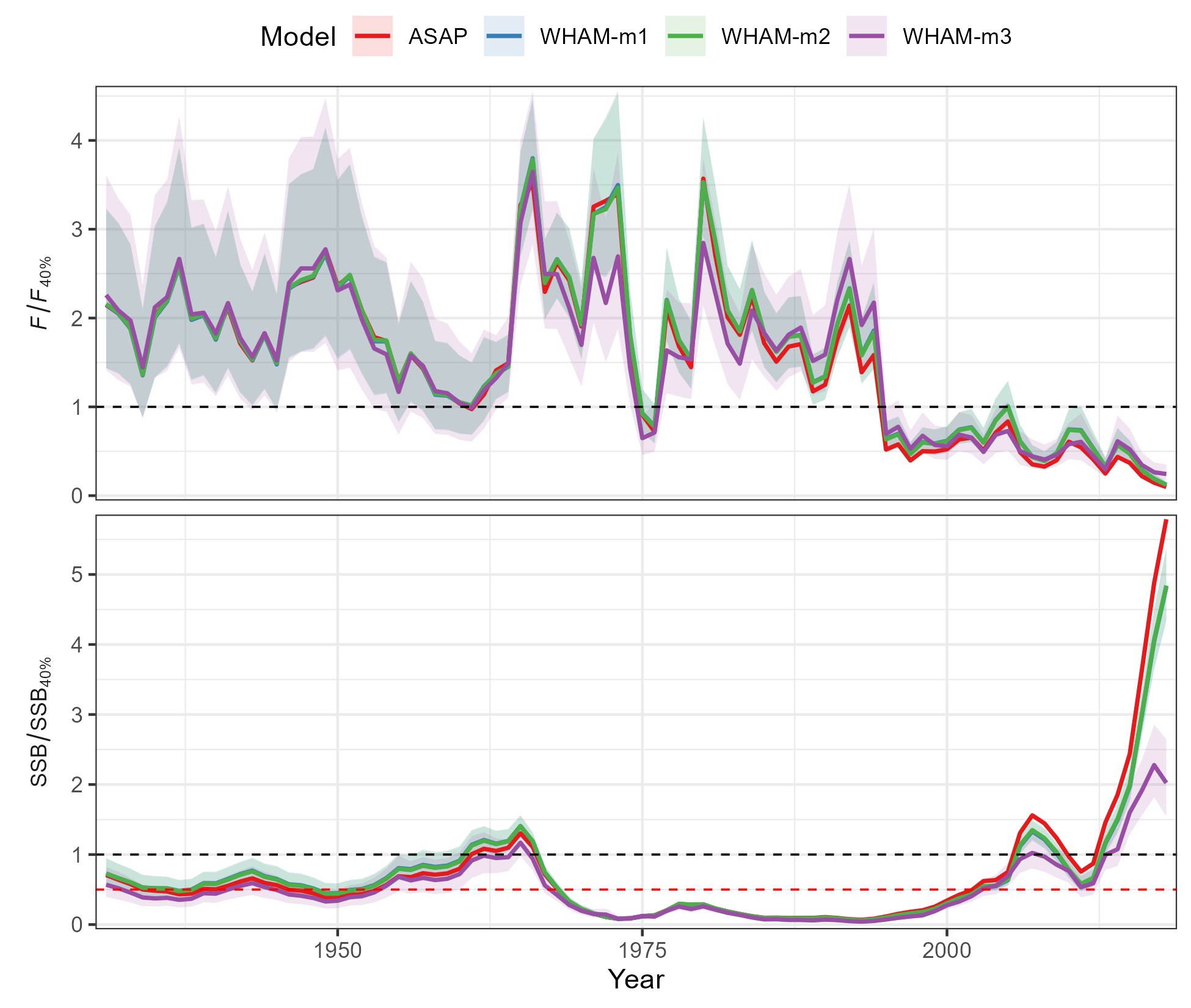
Note that even if you’re only making one plot using
$which, res$g is still a list of length 10.
For example, to plot SSB, F, and recruitment from 1980-2018 relative to
ASAP without confidence intervals:
res <- compare_wham_models(mods, do.table=F, plot.opts=list(years=1980:2018, ci=FALSE, relative.to="ASAP", which=1))
cols <- c("black", RColorBrewer::brewer.pal(n = 3, name = "Set1"))
res$g[[1]] + scale_colour_manual(values=cols)
ggsave(file.path(write.dir,"which1_relative_colorchange.png"), device='png', width=5, height=5.5, units='in')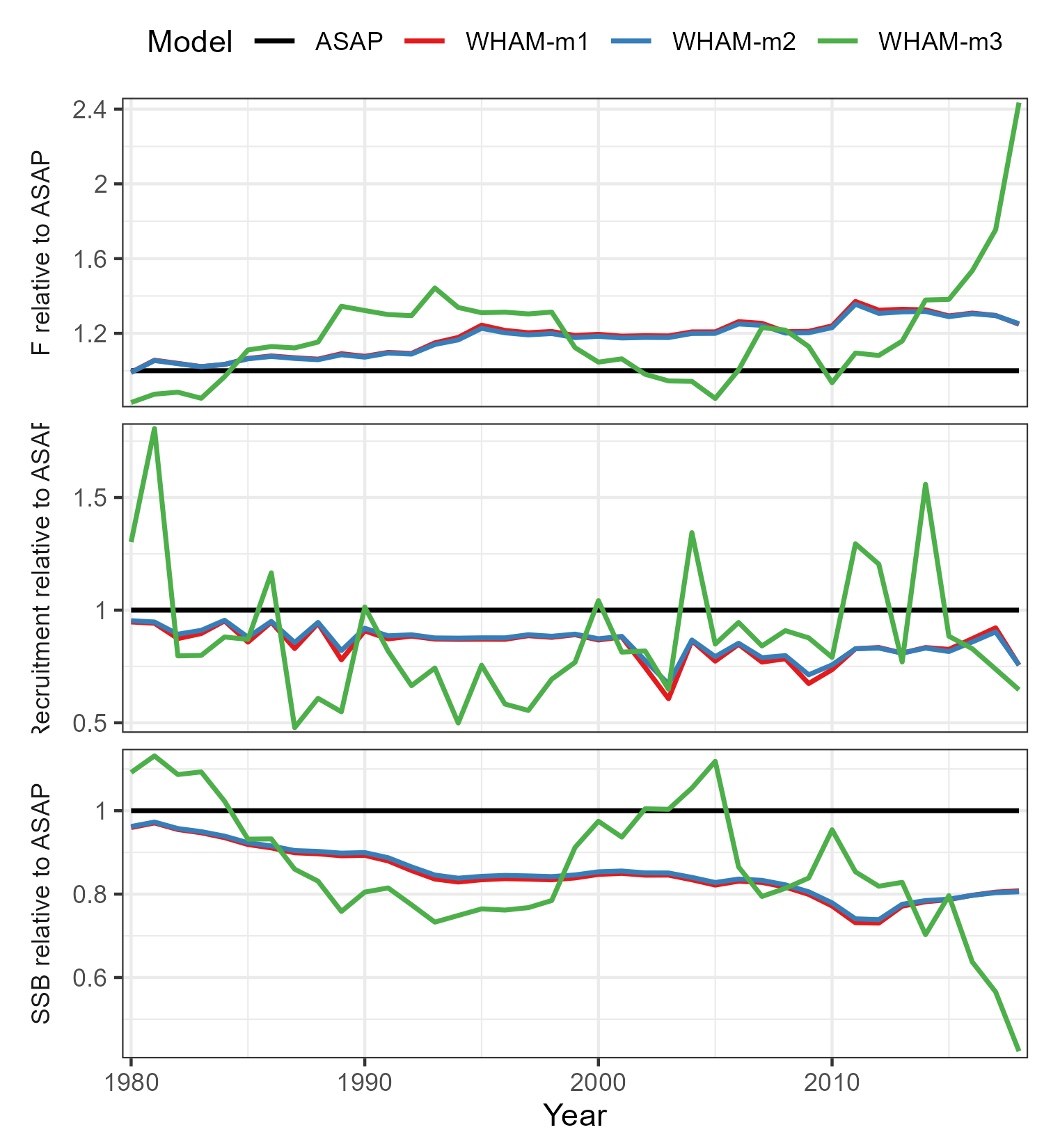
Any aesthetics that weren’t in the original plot are more complicated. For example, if we want to make the base model line dashed, linetype was not in original plot. We can do:
res$g[[1]]$mapping$linetype = quote(Model)
res$g[[1]]$labels$linetype = "Model"
ltys <- c(2,1,1,1)
res$g[[1]] + scale_colour_manual(values=cols) + scale_linetype_manual(values=ltys)
ggsave(file.path(write.dir,"which1_relative_colorchange_linetype.png"), device='png', width=5, height=5.5, units='in')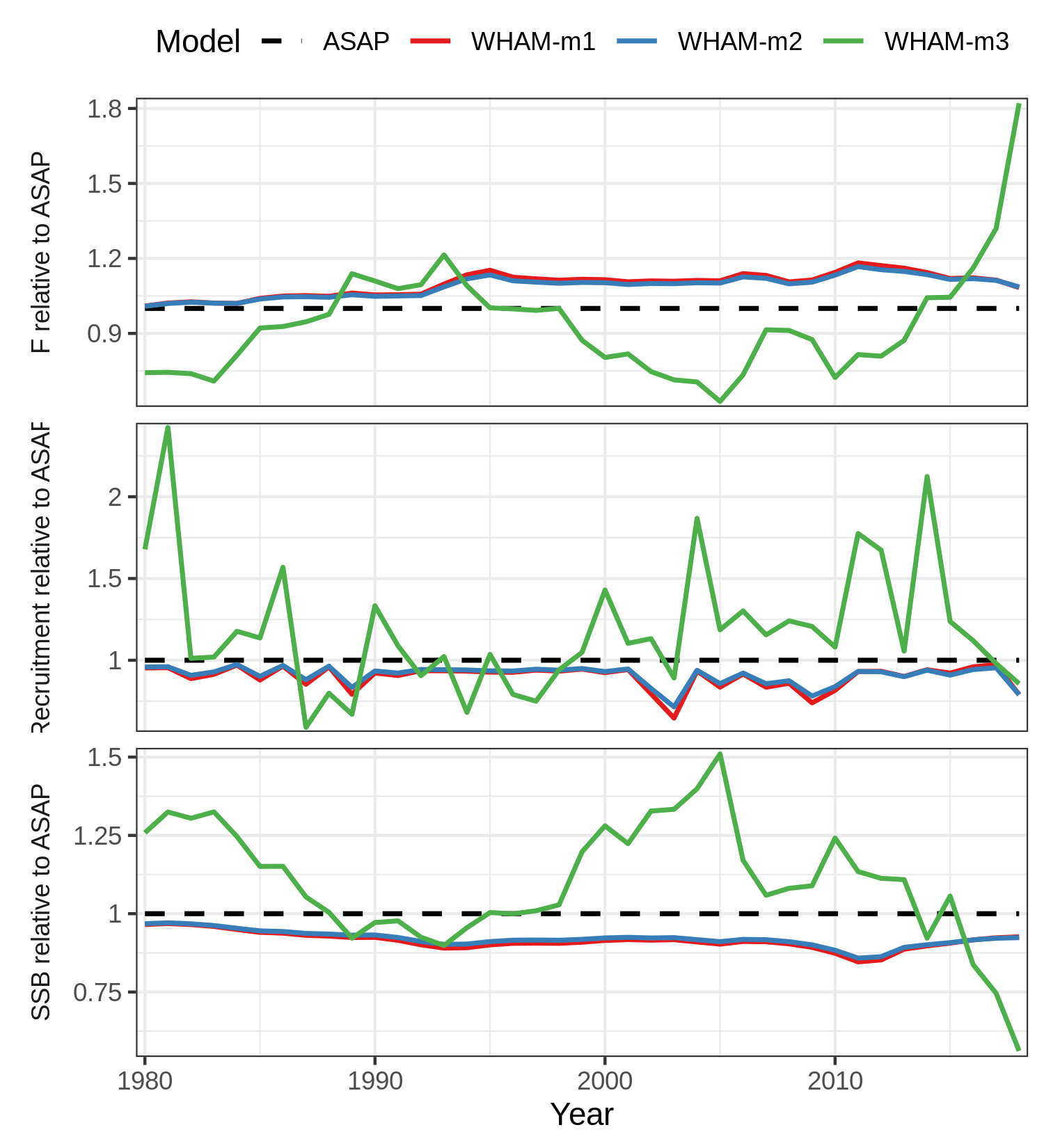
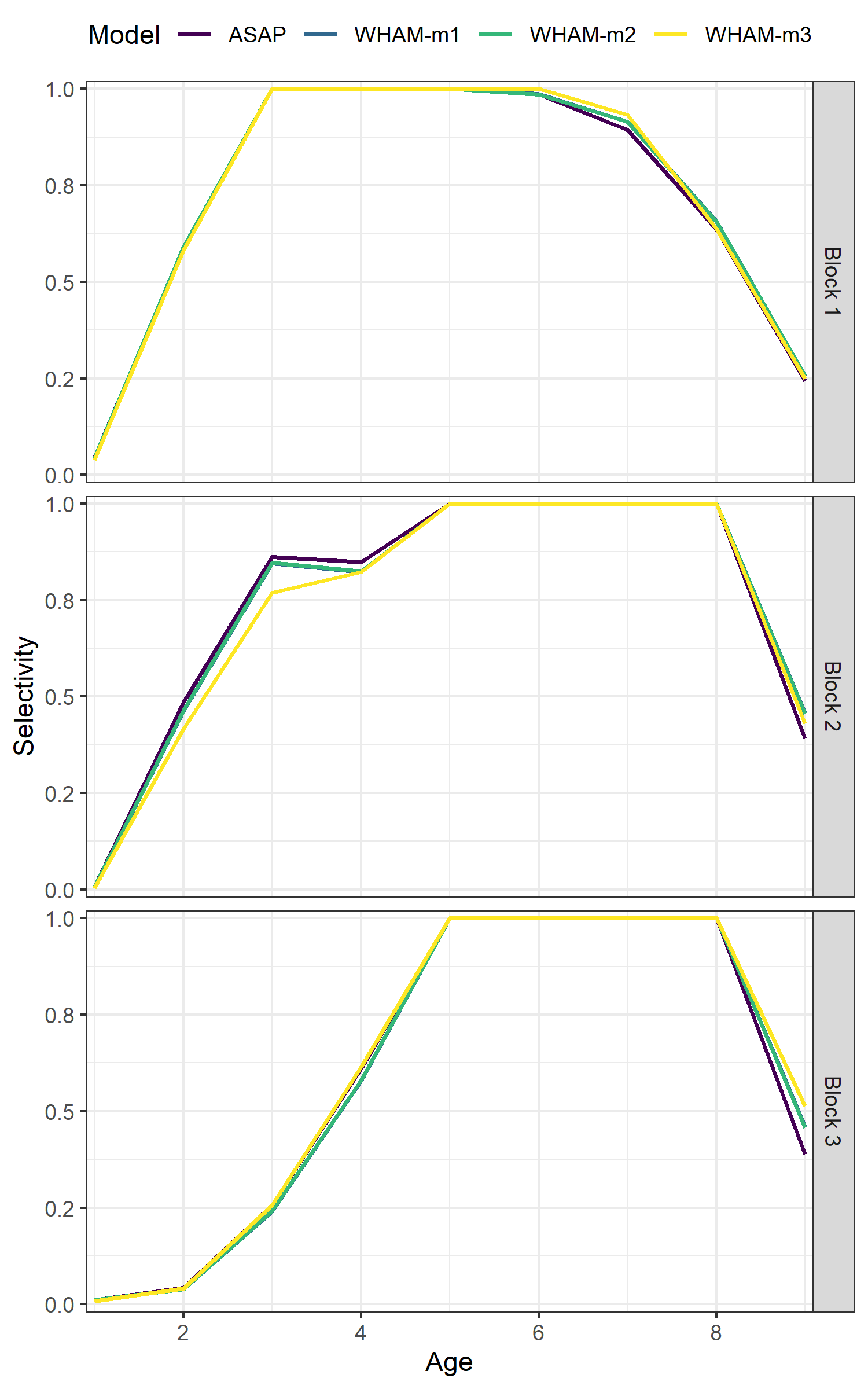
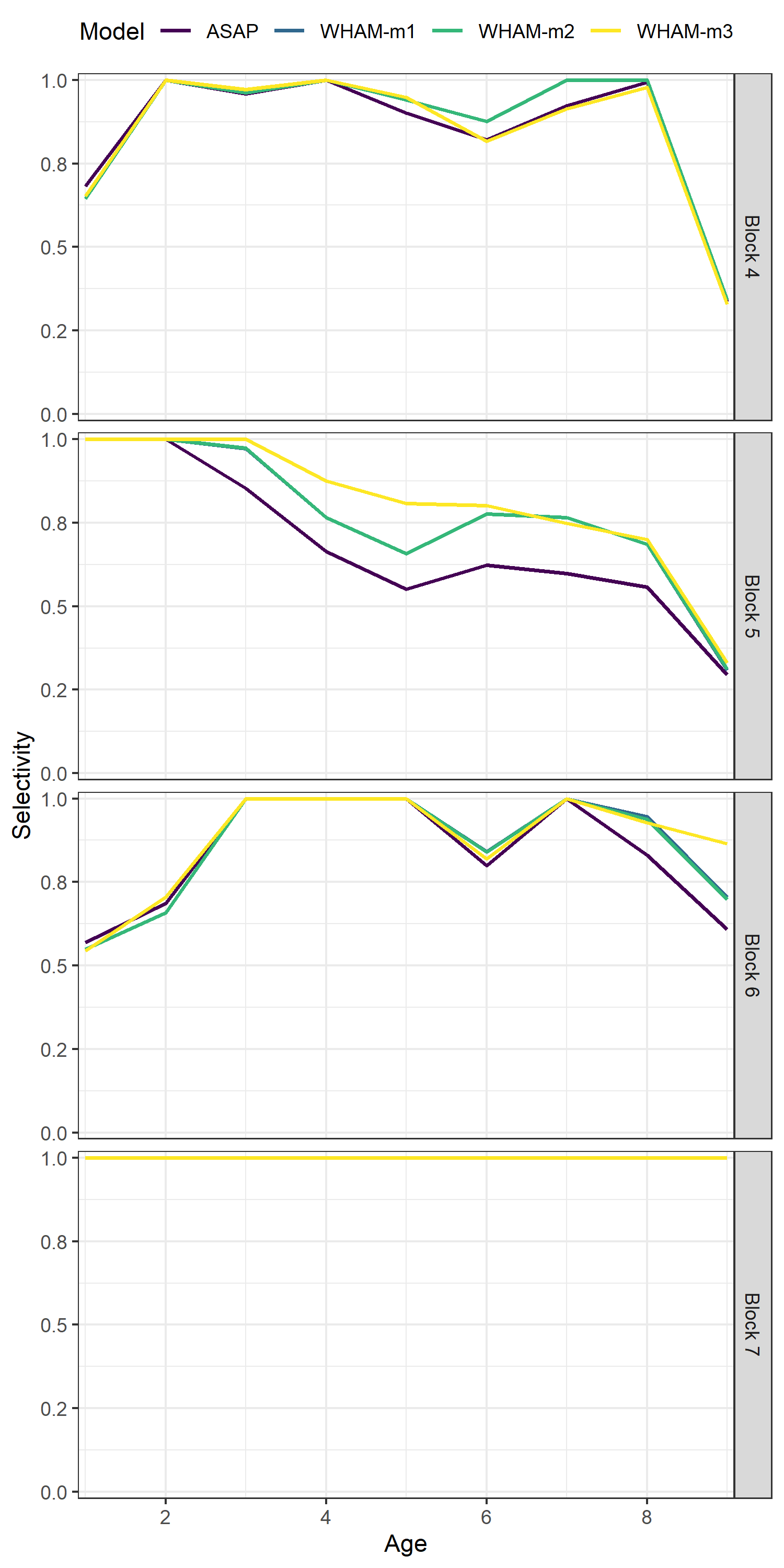
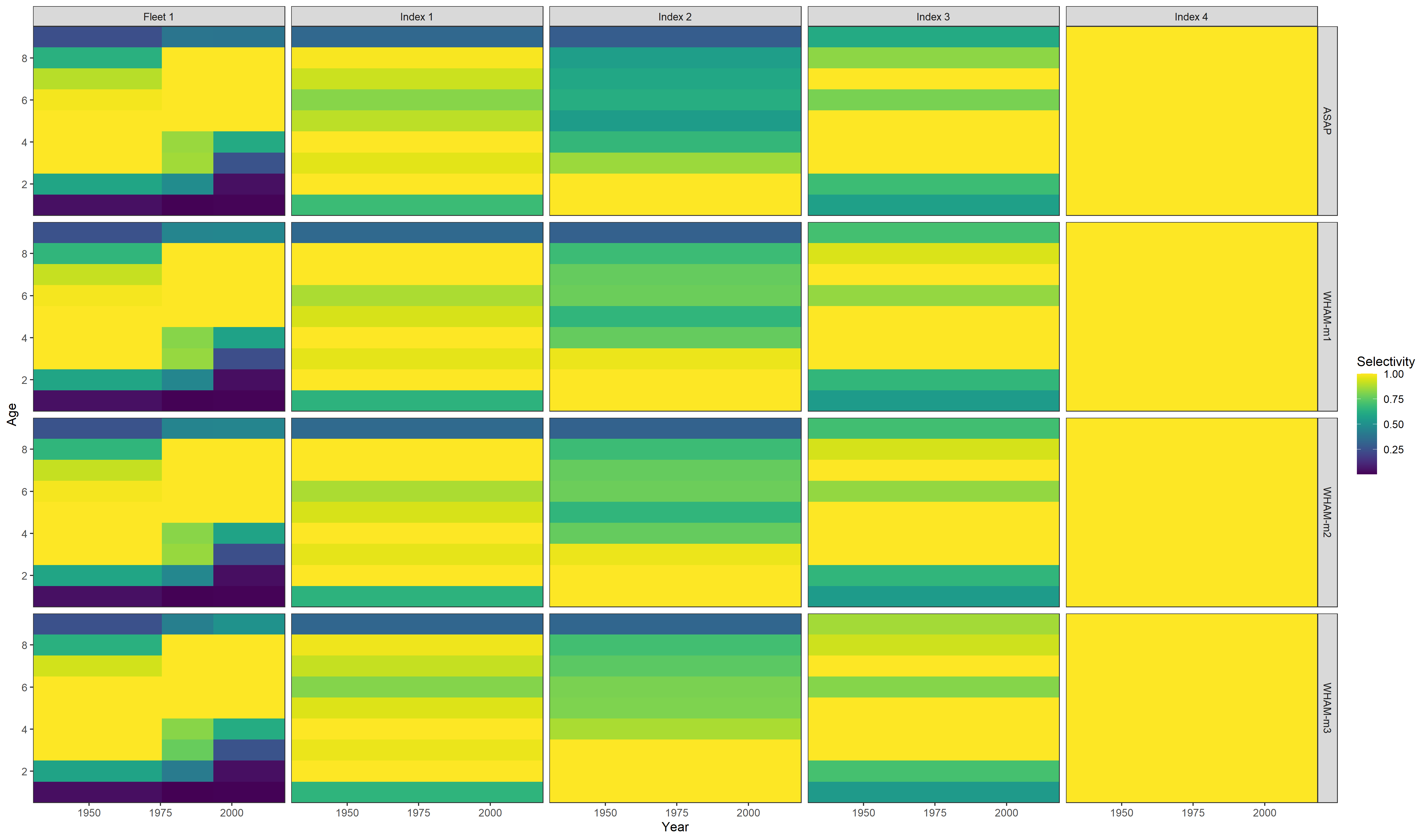
Our final example, changing the labels on the selectivity plot facets
res <- compare_wham_models(mods, do.table=F, plot.opts=list(which=4))
index_names <- as_labeller(c(`Block 4` = "NEFSC - Spring", `Block 5` = "NEFSC - Fall",`Block 6` = "DFO", `Block 7` = "NEFSC - Spring41"))
res$g[[4]] + facet_wrap(vars(Block), ncol=1, strip.position = 'right', labeller = index_names)
ggsave(file.path(write.dir,"which4_labels.png"), device='png', width=4.5, height=5.5, units='in')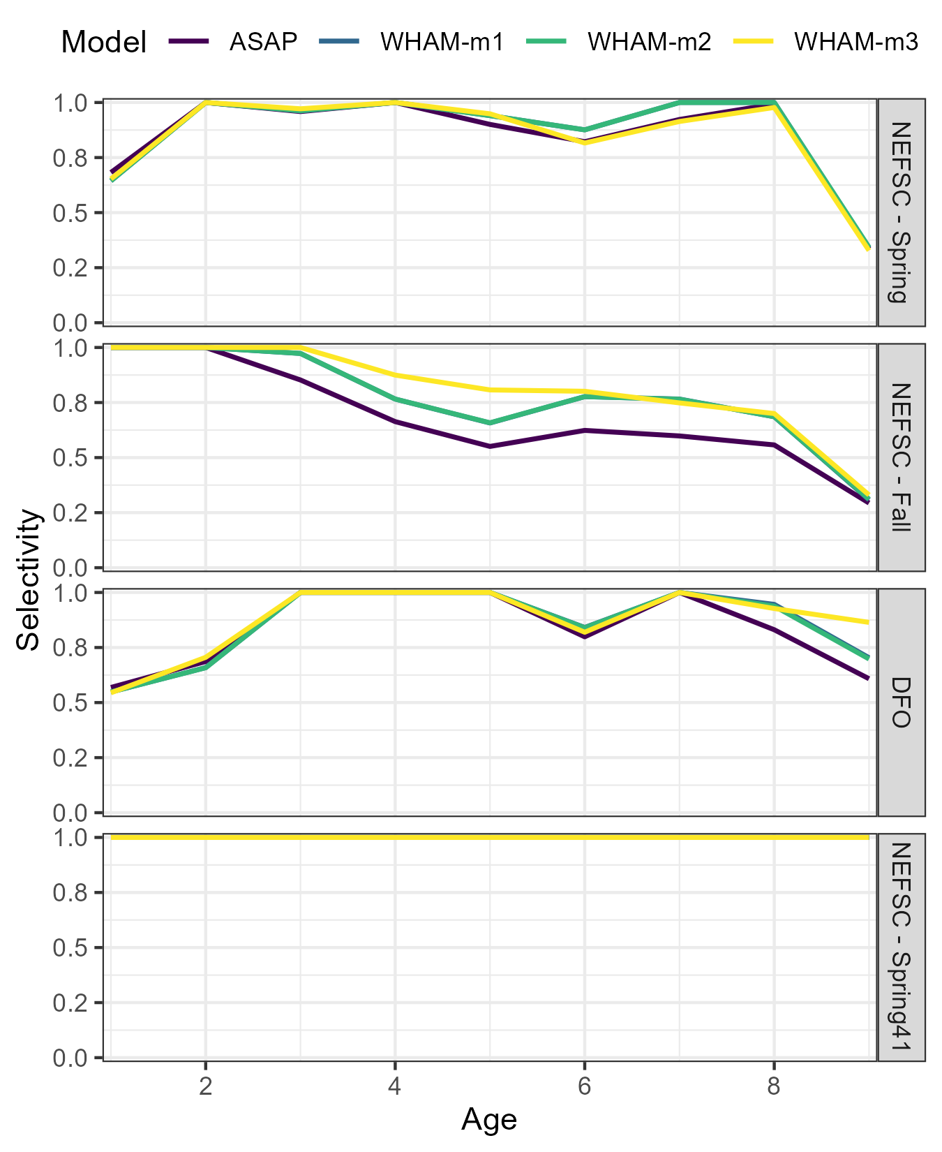
Hopefully that is enough to get you started!