Ex 4: Selectivity with time- and age-varying random effects
Source:vignettes/ex04_selectivity.Rmd
ex04_selectivity.RmdIn this vignette we walk through an example using the
wham (WHAM = Woods Hole Assessment Model) package to run a
state-space age-structured stock assessment model. WHAM is a
generalization of code written for Miller et al. (2016)
and Xu et
al. (2018), and in this example we apply WHAM to the same stock,
Southern New England / Mid-Atlantic Yellowtail Flounder.
Here we assume you already have wham installed. If not,
see the Introduction.
This is the 4th wham example, which builds off model
m4 from example
1:
full state-space model (numbers-at-age are random effects for all ages,
NAA_re = list(sigma='rec+1',cor='iid'))logistic normal age compositions, treating observations of zero as missing (
age_comp = "logistic-normal-miss0")random-about-mean recruitment (
recruit_model = 2)no environmental covariate (
ecov = NULL)2 indices
fit to 1973-2016 data
In example 4, we demonstrate the time-varying selectivity options in WHAM for both logistic and age-specific selectivity:
none: time-constantiid: parameter- and year-specific (random effect) deviations from mean selectivity parametersar1: as above, but estimate correlation across logistic parametersar1_y: as above, but estimate correlation across years2dar1: as above, but estimate correlation across both years and parameters
Note that each of these options can be applied to any selectivity block (and therefore fleet/catch or index/survey).
1. Load data
Open R and load the wham package:
For a clean, runnable .R script, look at
ex4_selectivity.R in the example_scripts
folder of the wham package. You can run this entire example
script with:
wham.dir <- find.package("wham")
source(file.path(wham.dir, "example_scripts", "ex4_selectivity.R"))
Let’s create a directory for this analysis:
# choose a location to save output, otherwise will be saved in working directory
write.dir <- "choose/where/to/save/output" # need to change e.g., tempdir(check=TRUE)
dir.create(write.dir)
setwd(write.dir)
We need the same data files as in example
1. Read in ex1_SNEMAYT.dat:
asap3 <- read_asap3_dat(file.path(wham.dir,"extdata","ex1_SNEMAYT.dat"))2. Specify selectivity model options
We are going to run 8 models that differ only in the selectivity options:
# m1-m5 logistic, m6-m9 age-specific
sel_model <- c(rep("logistic",3), rep("age-specific",5))

# time-varying options for each of 3 blocks (b1 = fleet, b2-3 = indices)
sel_re <- list(c("none","none","none"), # m1-m4 logistic
                c("iid","none","none"),
#               c("ar1","none","none"), #can't get a converged model for logistic with two re and two fe for
                c("2dar1","none","none"),
                c("none","none","none"), # m4-m8 age-specific
                c("iid","none","none"),
                c("ar1","none","none"), #will map all age-specific (mean) parameters to one estimated value
                c("ar1_y","none","none"),
                c("2dar1","none","none"))
n.mods <- length(sel_re)

# summary data frame
df.mods <- data.frame(Model=paste0("m",1:n.mods),
    Selectivity=sel_model, # Selectivity model (same for all blocks)
    Block_1_re=sapply(sel_re, function(x) x[[1]])) # Block 1 random effects
rownames(df.mods) <- NULL

df.mods
#>   Model  Selectivity Block_1_re
#> 1    m1     logistic       none
#> 2    m2     logistic        iid
#> 3    m3     logistic      2dar1
#> 4    m4 age-specific       none
#> 5    m5 age-specific        iid
#> 6    m6 age-specific        ar1
#> 7    m7 age-specific      ar1_y
#> 8    m8 age-specific      2dar1
3. Setup and run models
The ASAP data file specifies selectivity options (model, initial
parameter values, which parameters to fix/estimate). WHAM uses these by
default in order to facilitate running ASAP models. To see the currently
specified selectivity options in asap3:
asap3$dat$sel_block_assign # 1 fleet, all years assigned to block 1
#> NULL
# by default each index gets its own selectivity block (here, blocks 2 and 3)

asap3$dat$sel_block_option # fleet selectivity (1 block), 2 = logistic
#> NULL
asap3$dat$index_sel_option # index selectivity (2 blocks), 2 = logistic
#> NULL

asap3$dat$sel_ini # fleet sel initial values (col1), estimation phase (-1 = fix)
#> NULL
asap3$dat$index_sel_ini # index sel initial values (col1), estimation phase (-1 = fix)
#> NULL
When we specify the WHAM model with
prepare_wham_input(), we can overwrite the selectivity
options from the ASAP data file with the optional list argument
selectivity. The selectivity model is chosen via
selectivity$model:
| Model | selectivity$model |
No. Parameters |
|---|---|---|
| Age-specific | "age-specific" |
n_ages |
| Logistic (increasing) | "logistic" |
2 |
| Double logistic (dome) | "double-logistic" |
4 |
| Logistic (decreasing) | "decreasing-logistic" |
2 |
Regardless of the selectivity model used, we incorporate time-varying selectivity by estimating a mean for each selectivity parameter, , and (random effect) deviations from the mean, . We then estimate the selectivity parameters, , on the logit-scale with (possibly) lower and upper limits:
The deviations, , follow a 2-dimensional AR(1) process defined by the parameters , , and :
Mean selectivity parameters can be initialized at different values
from the ASAP file with selectivity$initial_pars.
Parameters can be fixed at their initial values by specifying
selectivity$fix_pars. Finally, we specify any time-varying
(random effects) on selectivity parameters
(selectivity$re):
selectivity$re |
Deviations from mean | Estimated parameters |
|---|---|---|
"none" |
time-constant (no deviation) | |
"iid" |
independent, identically-distributed | |
"ar1" |
autoregressive-1 (correlated across ages/parameters) | , |
"ar1_y" |
autoregressive-1 (correlated across years) | , |
"2dar1" |
2D AR1 (correlated across both years and ages/parameters) | , , |
We will loop over and fit each of the models, but first lets define some initial parameter values and which will be fixed. This is needed specifically for the age-specific selectivity models.
#initial pars for logistic or age-specfic selectivity
initial_pars <- c(rep(list(list(c(2,0.3),c(2,0.3),c(2,0.3))),3), rep(list(list(c(0.1,0.5,0.5,1,1,1),c(0.5,0.5,0.5,1,1,0.5),c(0.5,0.5,1,1,1,1))),5))
#which pars to fix for age-specific selectivity
fix_pars <- c(list(NULL,NULL,NULL), rep(list(list(4:6,4:5,3:6)),5))
Now we can run the above models in a loop:
#make a list of fits to fill in
mods <- list()

for(m in 1:n.mods){
    # overwrite initial parameter values in ASAP data file (ex1_SNEMAYT.dat)
    input <- prepare_wham_input(asap3, model_name=paste(paste0("Model ",m), sel_model[m], paste(sel_re[[m]], collapse="-"), sep=": "), recruit_model=2,
                selectivity=list(model=rep(sel_model[m],3), re=sel_re[[m]], initial_pars=initial_pars[[m]], fix_pars = fix_pars[[m]]),
                NAA_re = list(sigma='rec+1',cor='iid'),
                age_comp = "logistic-normal-miss0") # logistic normal, treat 0 obs as missing

    # fit model
    mods[[m]] <- fit_wham(input, do.check=T, do.osa=F, do.retro=F)
}

#save the model fits
for(m in 1:length(mods)) saveRDS(mod[[m]], file=paste0("m",m,".rds"))
4. Model convergence and comparison
Check which models converged.
vign4_conv <- lapply(mods, function(x) capture.output(check_convergence(x)))
for(m in 1:n.mods) cat(paste0("Model ",m,":"), vign4_conv[[m]], "", sep='\n')
#> Model 1:
#> stats:nlminb thinks the model has converged: mod$opt$convergence == 0
#> Maximum gradient component: 6.24e-11
#> Max gradient parameter: log_NAA_sigma
#> TMB:sdreport() was performed successfully for this model
#>
#> Model 2:
#> stats:nlminb thinks the model has converged: mod$opt$convergence == 0
#> Maximum gradient component: 8.81e-13
#> Max gradient parameter: logit_q
#> TMB:sdreport() was performed successfully for this model
#>
#> Model 3:
#> stats:nlminb thinks the model has converged: mod$opt$convergence == 0
#> Maximum gradient component: 2.84e-13
#> Max gradient parameter: logit_q
#> TMB:sdreport() was performed successfully for this model
#>
#> Model 4:
#> stats:nlminb thinks the model has converged: mod$opt$convergence == 0
#> Maximum gradient component: 1.71e-10
#> Max gradient parameter: log_NAA_sigma
#> TMB:sdreport() was performed successfully for this model
#>
#> Model 5:
#> stats:nlminb thinks the model has converged: mod$opt$convergence == 0
#> Maximum gradient component: 5.27e-08
#> Max gradient parameter: catch_paa_pars
#> TMB:sdreport() was performed successfully for this model
#>
#> Model 6:
#> stats:nlminb thinks the model has converged: mod$opt$convergence == 0
#> Maximum gradient component: 5.61e-13
#> Max gradient parameter: logit_q
#> TMB:sdreport() was performed successfully for this model
#>
#> Model 7:
#> stats:nlminb thinks the model has converged: mod$opt$convergence == 0
#> Maximum gradient component: 1.08e-09
#> Max gradient parameter: index_paa_pars
#> TMB:sdreport() was performed successfully for this model
#>
#> Model 8:
#> stats:nlminb thinks the model has converged: mod$opt$convergence == 0
#> Maximum gradient component: 3.58e-09
#> Max gradient parameter: F_pars
#> TMB:sdreport() was performed successfully for this modelPlot output for models that converged (in a subfolder for each model):
# Is Hessian positive definite?
ok_sdrep = sapply(mods, function(x) if(x$na_sdrep==FALSE & !is.na(x$na_sdrep)) 1 else 0)
pdHess <- as.logical(ok_sdrep)
# did stats::nlminb converge?
conv <- sapply(mods, function(x) x$opt$convergence == 0) # 0 means opt converged
conv_mods <- (1:n.mods)[pdHess]
for(m in conv_mods){
    #html and png files by default
    plot_wham_output(mod=mods[[m]], dir.main=file.path(write.dir,paste0("m",m)))
}
Compare the models using AIC:
df.aic <- as.data.frame(compare_wham_models(mods, table.opts=list(sort=FALSE, calc.rho=FALSE))$tab)
df.aic[!pdHess,] = NA
minAIC <- min(df.aic$AIC, na.rm=T)
df.aic$dAIC <- round(df.aic$AIC - minAIC,1)
df.mods <- cbind(data.frame(Model=paste0("m",1:n.mods), Selectivity=sel_model,
                            "Block1_re"=sapply(sel_re, function(x) x[[1]]),
                            "opt_converged"= ifelse(conv, "Yes", "No"),
                            "pd_hessian"= ifelse(pdHess, "Yes", "No"),
                            "NLL"=sapply(mods, function(x) round(x$opt$objective,3)),
                            "Runtime"=sapply(mods, function(x) x$runtime)), df.aic)
rownames(df.mods) <- NULL
df.mods
#> Model Selectivity Block1_re opt_converged pd_hessian NLL Runtime dAIC
#> 1 m1 logistic none Yes Yes -788.748 0.73 54.5
#> 2 m2 logistic iid Yes Yes -811.603 0.87 10.8
#> 3 m3 logistic 2dar1 Yes Yes -818.980 0.89 0.0
#> 4 m4 age-specific none Yes Yes -793.497 0.67 51.0
#> 5 m5 age-specific iid Yes Yes -793.497 0.84 53.0
#> 6 m6 age-specific ar1 Yes Yes -785.042 0.85 67.9
#> 7 m7 age-specific ar1_y Yes Yes -818.610 0.68 4.8
#> 8 m8 age-specific 2dar1 Yes Yes -820.487 0.84 3.0
#> AIC
#> 1 -1449.5
#> 2 -1493.2
#> 3 -1504.0
#> 4 -1453.0
#> 5 -1451.0
#> 6 -1436.1
#> 7 -1499.2
#> 8 -1501.0Prepare to plot selectivity-at-age for block 1 (fleet).
library(tidyverse)
library(viridis)

selAA <- lapply(mods, function(x) x$report()$selAA[[1]])
sel_mod <- factor(c("Age-specific","Logistic")[sapply(mods, function(x) x$env$data$selblock_models[1])], levels=c("Logistic","Age-specific"))
sel_cor <- factor(c("None","IID","AR1","AR1_y","2D AR1")[sapply(mods, function(x) x$env$data$selblock_models_re[1])], levels=c("None","IID","AR1","AR1_y","2D AR1"))
df.selAA <- data.frame(matrix(NA, nrow=0, ncol=11))
colnames(df.selAA) <- c(paste0("Age_",1:6),"Year","Model","conv","sel_mod","sel_cor")
for(m in 1:n.mods){
    df <- as.data.frame(selAA[[m]])
    df$Year <- input$years
    colnames(df) <- c(paste0("Age_",1:6),"Year")
    df$Model <- m
    df$conv <- ifelse(df.mods$pd_hessian[m]=="Yes",1,0)
    df$sel_mod = sel_mod[m]
    df$sel_cor = sel_cor[m]
    df.selAA <- rbind(df.selAA, df)
}
df <- df.selAA |> pivot_longer(-c(Year,Model,conv,sel_mod,sel_cor),
                names_to = "Age",
                names_prefix = "Age_",
                names_transform = list(Age = as.integer),
                values_to = "Selectivity")
df$Age <- as.integer(df$Age)
df$sel_mod <- factor(df$sel_mod, levels=c("Logistic","Age-specific"))
df$sel_cor <- factor(df$sel_cor, levels=c("None","IID","AR1","AR1_y","2D AR1"))
df$conv = factor(df$conv)
Now plot selectivity-at-age for block 1 (fleet) in all models.
print(ggplot(df, aes(x=Year, y=Age)) +
    geom_tile(aes(fill=Selectivity)) +
    geom_label(aes(x=Year, y=Age, label=lab), size=5, alpha=1, #fontface = "bold",
      data=data.frame(Year=1975.5, Age=5.8, lab=paste0("m",1:length(mods)), sel_mod=sel_mod, sel_cor=sel_cor)) +
    facet_grid(rows=vars(sel_cor), cols=vars(sel_mod)) +
    scale_fill_viridis() +
    theme_bw() +
    scale_x_continuous(expand=c(0,0)) +
    scale_y_continuous(expand=c(0,0)))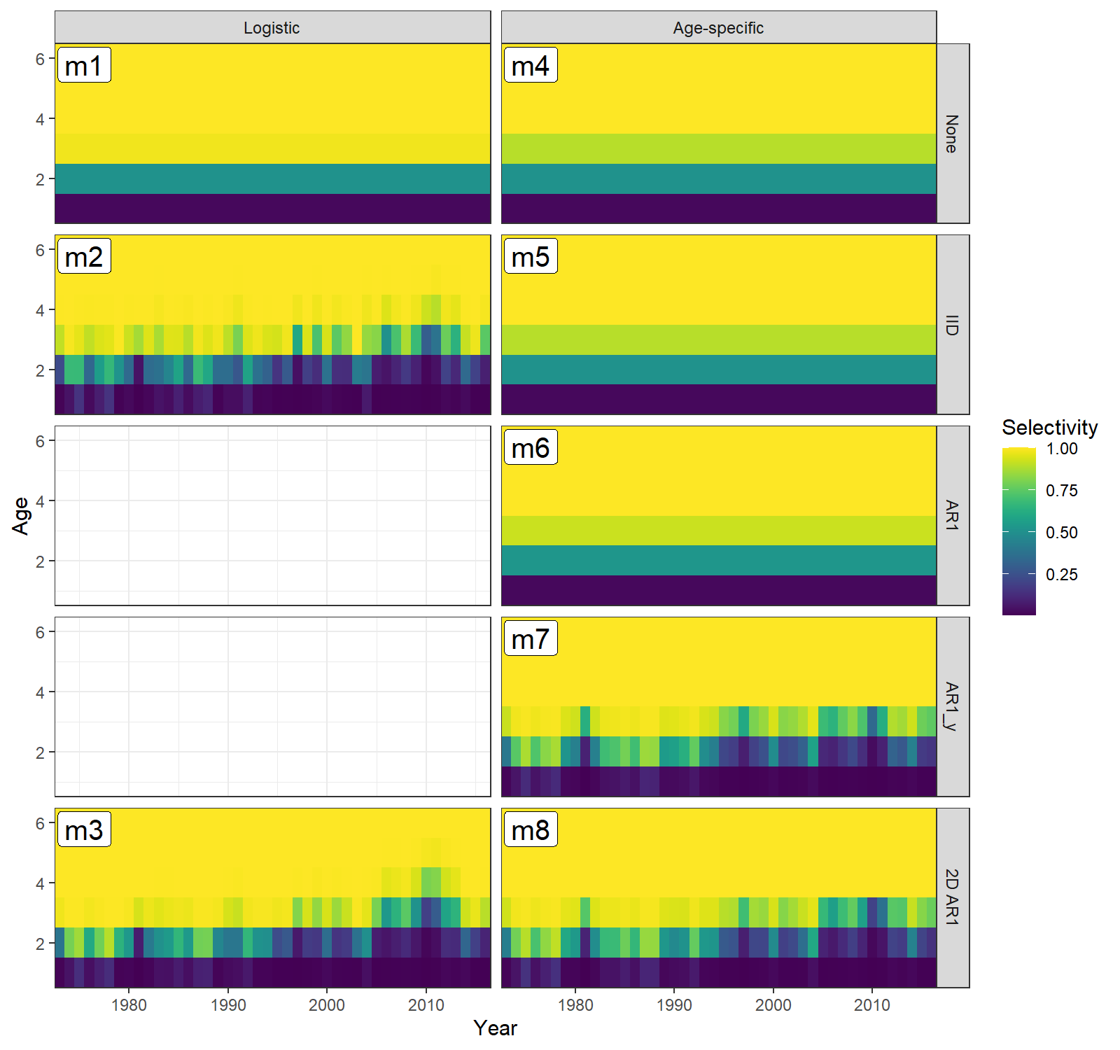
A note on convergence
When fitting age-specific selectivity, oftentimes some of the (mean, ) selectivity parameters need to be fixed for the model to converge. The specifications used here follow this procedure:
- Fit the model without fixing any selectivity parameters.
- If the model fails to converge or the hessian is not invertible
(i.e. not positive definite), look for mean selectivity parameters that
are very close to 0 or 1 (> 5 or < -5 on the logit scale) and/or
have
NaNestimates of their standard error:
mod$parList$logit_selpars # mean sel pars
mod$input$map$sel_repars # if time-varying selectivity turned on
mod$rep$selAA # list of annual selectivity-at-age by block
mod$sdrep # look for sel pars with NaN standard errors- Re-run the model fixing the worst selectivity-at-age parameter for each block at 0 or 1 as appropriate. In the above age-specific models, we initially just fixed age 4 in block 2. The logit scale selectivity for age 5 for that block was around 20 for at least one model, indicating that they too should be fixed at 1. Sometimes just initializing the worst parameter is enough, without fixing it.
- The goal is to find a set of selectivity parameter initial/fixed values that allow all nested models to converge. Fixing parameters should not affect the NLL much, and any model that is a superset of another should not have a greater NLL (indicates not converged to global minimum). The following commands may be helpful: